8 Appendix
This chapter is primarily based on:
- Casella, G., & Berger, R. L. (2002). Statistical inference (Vol. 2). Pacific Grove, CA: Duxbury (chapters 1 & 3).
8.1 Random Variables & Probability Distributions
8.1.1 Random variables
8.1.1.1 Why Random Variables?
Random variables are used to extract and simplify information that we obtain from an experiment. For example, if we toss five coins it would be tedious to say “I have observed heads, heads, tails, heads, tails”. With five coins this might still be a feasible way to convey the outcome of the experiment, but what about 500 coins? Instead, we naturally condense the information into a random variable (even though we might not call it that) and say “I have observed three heads” or we define another random variable and say “I have observed two tails”. There are many ways to summarize the outcome of an experiment and hence we can define multiple random variables from the same experiment. We could also define a more “complicated” random variable that adds four points for each heads and one point for each tails. In general there are no restrictions on our function as long as it maps from the sample space to the real numbers. We distinguish two types of random variables, discrete and continuous, which are discussed in the following sections.
8.1.1.2 Tossing coins
As a first example of a random variable, assume you toss a chosen number of coins (between 1 and 20). The tossing is the experiment in this case. The sample space consists of all the possible combinations of heads (“h”) and tails (“t”) given the number of coins. For a single coin:
\[ S = \{h, t\} \]
For two coins:
\[ S = \{hh, ht, th, tt\} \]
For three coins:
\[ S = \{hhh, hht, hth, thh, tth, tht, htt, ttt\} \]
and so on.
One of the outcomes in the sample space will be realized whenever one tosses the coin(s). The definition of random variables allows for many possibilities. An operation that takes any realization of the experiment (e.g. hht) as an input and gives us a real number as an outcome is a random variable. For this example we have chosen “number of heads” as the function but it could also be number of tails or (number of heads)+(4*number of tails). Lets call our function \(g\). Then
\[ g(hhh) = 3 > g(hht) = g(hth) = g(thh) = 2 > g(tth) = g(tht) = g(htt) = 1 > g(ttt) = 0 \]
for three coins.
So far we have only considered the possible outcomes but not how likely they are. We might be interested in how likely it is to observe 2 or less heads when tossing three coins. Let’s first consider a fair coin. With a fair coin it is just as likely to get heads as it is tails. Formally
\[ p(h) = p(t) = 0.5 \]
By definition the probabilities have to add up to one. If you think of probabilities in percentages, this just expresses that with 100% certainty something happens. If we toss a coin we are certain that we get either heads or tails and thus for a fair coin the chance is 50/50. Below you will find an app where you can experiment with different numbers of coins and different probabilities.
If you set the slider to 3 and the probability of observing h (\(p(h)\)) to \(0.5\) the cumulative distribution function will update accordingly. The dots mean that at that point we are already at the higher probability and not on the line below. Let’s analyze the result. The probability of observing less than or equal to 0 heads lies between 0 and 0.2. Of course we cannot observe a negative number of heads and so this is just the probability of observing no heads. There is only one realization of our experiment that fulfills that property: \(g(ttt) = 0\). So how likely is that to happen? Each coin has the probability 0.5 to show tails and we need all of them to land on tails. \[ p(ttt) = 0.5 * 0.5 * 0.5 = 0.125 \]
Another way of calculating the probability is to look at the sample space. There are 8 equally likely outcomes (for fair coins!) one of which fulfills the property that we observe 0 heads.
\[ p(ttt) = \frac{1}{8} = 0.125 = F_x(0) \]
The next “level” shows the probability of observing less than or equal to 1 head. That is the probability of observing 0 heads (\(p(ttt) = 0.125\)) plus the probability of observing one head (\(p(htt) + p(tht) + p(tth)\)). The probability of observing one head is given by the sum of the probabilities of the possibilities from the sample space. Let’s take a second to think about how probabilities are combined. If we want to know the probability of one event and another we have to multiply their respective probabilities such as in the case of \(p(ttt)\). There we wanted to know how likely it is that the first and the second and the third coin are all tails. Now we want to know the probability of either \(p(ttt)\) or \(p(htt)\) or \(p(tht)\) or \(p(tth)\). In the case that either event fulfills the condition we add the probabilities. This is possible because the probabilities are independent. That is, having observed heads (or tails) on the first coin does not influence the probability of observing heads on the others.
\[ p(ttt) = p(htt) = \underbrace{0.5}_{p(h)} * \underbrace{0.5}_{p(t)} *\underbrace{0.5}_{p(t)} = p(tht) = p(tth)= 0.125 \\ \Rightarrow F_X(1) = \underbrace{0.125}_{p(ttt) = F_X(0)} + \underbrace{0.125}_{p(htt)} + \underbrace{0.125}_{p(tht)} + \underbrace{0.125}_{p(tth)} = 0.5 \]
Now 4 out of the 8 possibilities (50%) in the sample space fulfill the property.
For \(F_X(2)\) we add the probabilities of the observing 2 heads (\(p(hht) + p(hth) + p(thh)\)).
\[ F_X(2) = \underbrace{0.5}_{F_X(1)} + \underbrace{0.125}_{p(hht)} + \underbrace{0.125}_{p(hth)} + \underbrace{0.125}_{p(thh)} = 0.875 = \frac{7}{8} \]
Since we are interested in less than or equal to we can always just add the probabilities of the possible outcomes at a given point to the cumulative distribution of the previous value (this gives us an idea about the link between cumulative distribution and probability mass functions). Now 7 out of 8 outcomes fulfill the property.
Obviously the probability of observing 3 or less heads when tossing 3 coins is 1 (the certain outcome).
This analysis changes if we consider a weighted coin that shows a higher probability on one side than the other. As the probability of observing heads increases the lines in the cumulative distribution shift downward. That means each of the levels are now less likely. In order to see why, let’s look at the probability of observing 2 or less heads when the probability of observing head is 0.75 (the probability of tails is thus 0.25) for each of the 3 coins.
\[ F_X(2) = \overbrace{\underbrace{0.25*0.25*0.25}_{p(ttt) = F_X(0) = 0.016} + \underbrace{0.75 * 0.25 * 0.25}_{p(htt)=0.047} + \underbrace{0.25 * 0.75 * 0.25}_{p(tht)=0.047} + \underbrace{0.25 * 0.25 * 0.75}_{p(tth)=0.047}}^{F_X(1) = 0.156}\dots\\ + \underbrace{0.75 * 0.75 * 0.25}_{p(hht) = 0.141} + \underbrace{0.75 * 0.25 * 0.75}_{p(hth) = 0.141} + \underbrace{0.25 * 0.75 * 0.75}_{p(thh) = 0.141} = 0.578 \]
What happens if you decrease the probability of observing heads?
The probability mass function defines the probability of observing an exact amount of heads (for all amounts) given the number of coins and the probability of observing heads. Continuing our example with 3 fair coins this means that \(f_X(0) = p(ttt) = 0.125\), \(f_X(1) = p(htt) + p(tht) + p(tth) = 0.375\), \(f_X(2) = p(hht) + p(hth) + p(thh) = 0.375\) and \(f_X(3) = p(hhh) = 0.125\). So instead of summing up the probabilities up to a given point we look at each point individually. This is also the link between the probability mass function and the cumulative distribution function: The cumulative distribution function at a given point (\(x\)) is just the sum of the probability mass function up to that point. That is
\[ F_X(0) = f_X(0),\ F_X(1) = f_X(0) + f_X(1),\ F_X(2) = f_X(0) + f_X(1) + f_X(2),\ \dots\\ F_X(x) = f_X(0) + f_X(1) + \dots + f_X(x) \]
A more general way to write this is:
\[ F_X(x) = \sum_{i=0}^x f_X(i) \]
8.1.1.3 Sum of two dice
Another example for a discrete random variable is the sum of two dice throws. Assume first that you have a six sided die. The six values it can take are all equally probable (if we assume that it is fair). Now if we throw two six sided dice and sum up the displayed dots, the possible values are no longer all equally probable. This is because some values can be produced by more combinations of throws. Consider the value 2. A 2 can only be produced by both dice displaying one dot. As the probability for a specific value on one die is \(\frac{1}{6}\), the probability of both throws resulting in a 1 is \(\frac{1}{6} * \frac{1}{6} = \frac{1}{36}\). Now consider the value 3. 3 can be produced by the first dice roll being a 1 and the second being a 2 and by the first roll being a 2 and the second a 1. While these may seem like the same thing, they are actually two distinct events. To calculate the probability of a 3 you sum the probabilities of these two possibilities together, i.e. \(P\{1,2\} + P\{2,1\} = \frac{1}{6} * \frac{1}{6} + \frac{1}{6} * \frac{1}{6} = \frac{2}{36}\). This implies that a 3 is twice as probable as a 2. When done for all possible values of the sum of two dice you arrive at the following probabilities:
\[ P(x) = \begin{cases} \frac{1}{36} & \text{if }x = 2 \text{ or } 12 \\ \frac{2}{36} = \frac{1}{18} & \text{if } x = 3 \text{ or } 11\\ \frac{3}{36} = \frac{1}{12} & \text{if } x = 4 \text{ or } 10\\ \frac{4}{36} = \frac{1}{9} & \text{if } x = 5 \text{ or } 11\\ \frac{5}{36} & \text{if } x = 6 \text{ or } 8\\ \frac{6}{36} = \frac{1}{6} & \text{if } x = 7\\ \end{cases} \]
To see what this looks like in practice you can simulate dice throws below. The program randomly throws two (or more) dice and displays their sum in a histogram with all previous throws. The longer you let the simulation run, the more the sample probabilities will converge to the theoretically calculated values above.
8.1.1.4 Discrete Random Variables
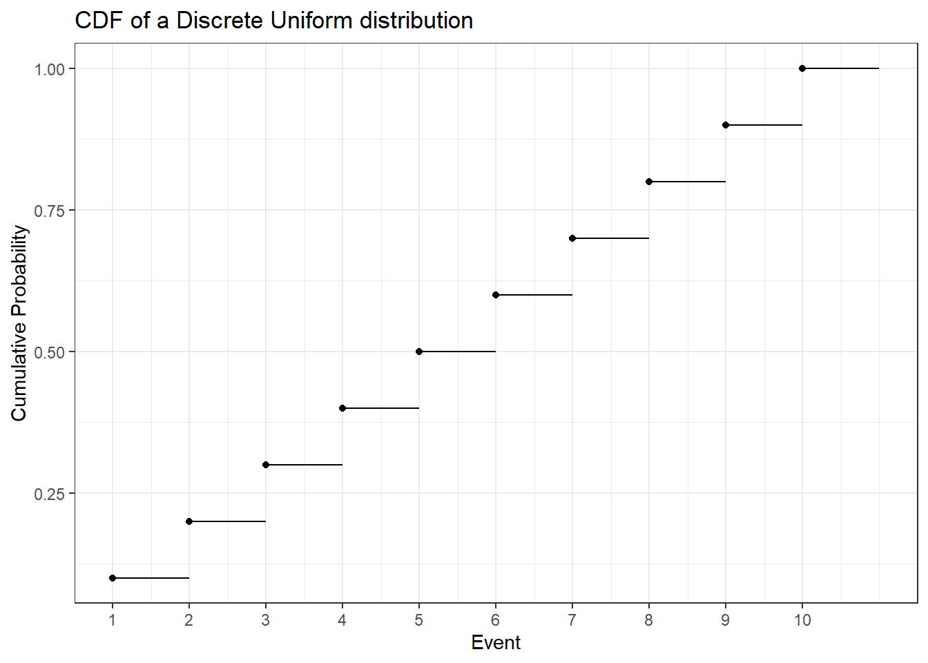
Now that we have seen examples for discrete random variables, we can define them more formally. A random variable is discrete if its cumulative distribution function is a step function as in the plot below. That is, the CDF shifts or jumps from one probability to the next at some point(s). Notice that the black dots indicate that at that specific point the probability is already at the higher step. More formally: the CDF is “right-continuous”. That is the case for all CDFs. To illustrate this concept we explore the plot below. We have a discrete random variable as the CDF jumps rather than being one line. We can observe integer values between 0 and 10 whereas the probability of observing less than or equal to 0 is almost 0 and the probability of observing less than or equal to 10 is 1. The function is right continuous: Let’s look at the values 4 and 5 for example. The probability of observing 4 or less than 4 is just under 0.4. The probability of observing 5 or less is just over 0.6. For further examples see tossing coins and sum of two dice
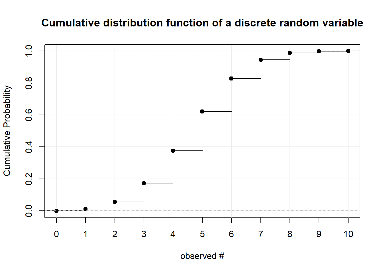
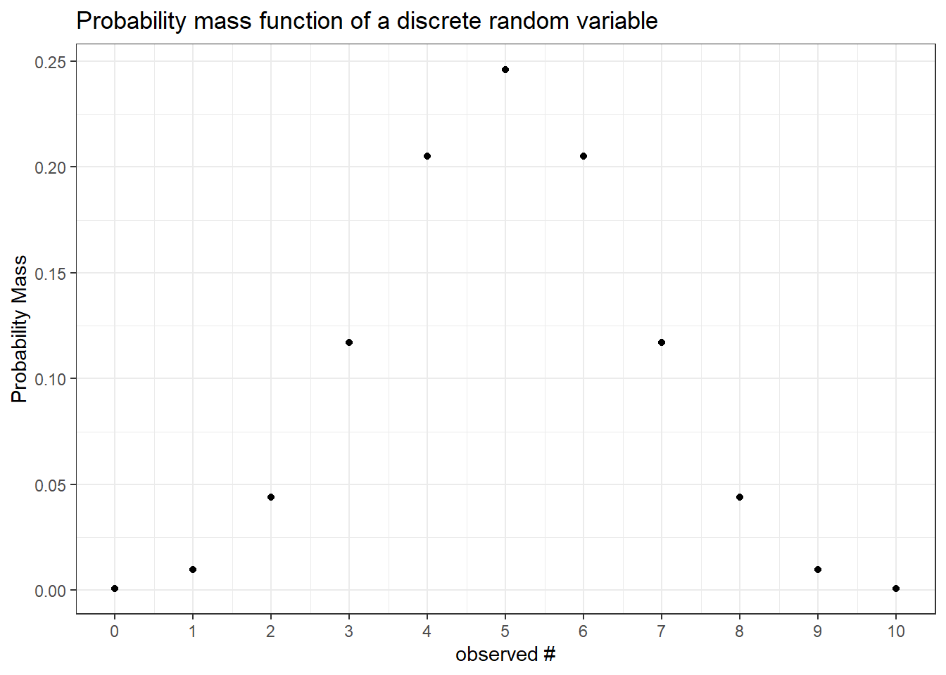
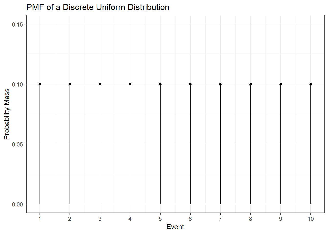
For discrete random variables the function that defines the probability of each event is called the probability mass function. Notice that the “jumps” in the CDF are equivalent to the mass at every point. It follows that the sum of the mass up to a point in the PMF (below) is equal to the level at that point in the CDF (above).
8.1.1.5 Continuous Case
The vigilant reader might have noticed that while the definition of a random variable allows for the function to map to the real numbers the coin and dice examples only uses mapping to the natural numbers. Just as with discrete random variables we can define continuous random variables by their cumulative distribution function. As you might have guessed the cumulative distribution function of a continuous random variable is continuous, i.e. there are no jumps.
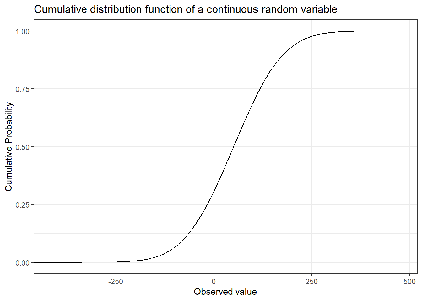
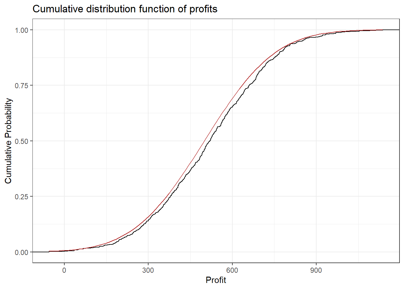
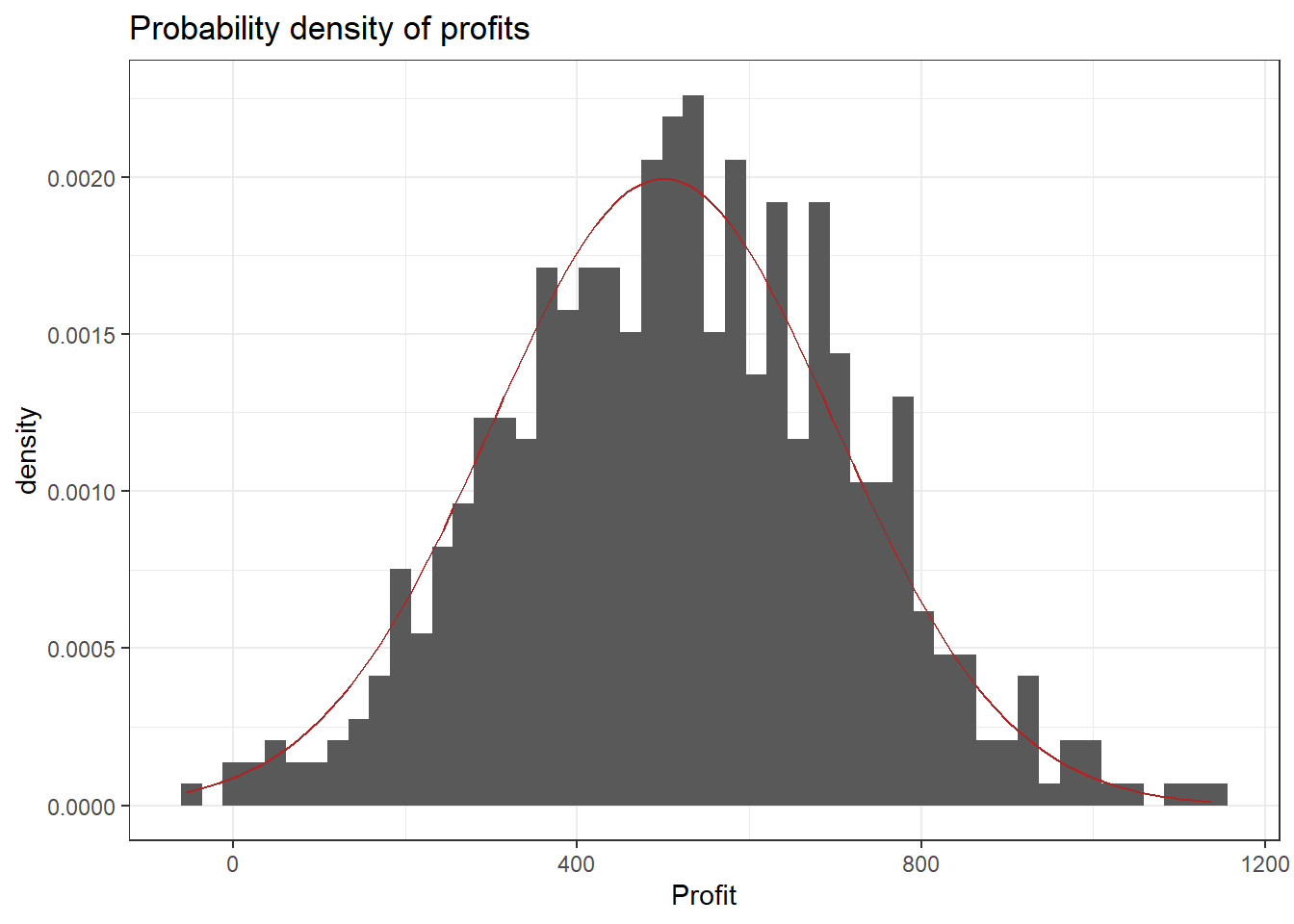
One example for a continuous random variable is the average profit of a store per week. Let’s think of the possible values: Profit could be negative if, for example, the payment to employees exceeds the contribution margin accrued from the products sold. Of course it can also be positive and technically it is not restricted to any range of values (e.g. it could exceed a billion, be below negative 10,000 or anywhere in between). Below you can see some (simulated) profit data. Observe that the CDF looks continuous. The red overlay is the CDF of the normal distribution (see chapter on probability distributions) which was used for the simulation. The final plot is a histogram of the data with the normal density (again in red). It shows that profits around 500 are more likely (higher bars) and the further away from 500 we get the less likely it is that a certain profit will be observed in a given week. Recall the definition of the probability density function shows the probability of a given outcome.
8.1.1.6 Definitions
Sample Space: The set of all possible outcomes of a particular experiment is called the sample space of the experiment (Casella & Berger, 2002, p. 1). Denoted \(S\).
Random Variable: A function from a sample space \(\left(S\right)\) into the real numbers (Casella & Berger, 2002, p. 27). Denoted \(X\).
Cumulative distribution function: A function that defines the probability that a random variable \(\left(X\right)\) is less than or equal to an outcome (\(x\)) for all possible outcomes (Casella & Berger, 2002, p. 29). Denoted
\[ F_X(x) = P_X(X \leq x), \text{ for all } x \]
Probability mass/density function: A function that defines the probability that a random variable \(\left(X\right)\) is equal to an outcome (\(x\)) for all possible outcomes. Denoted
\[ f_X(x)=P(X = x), \text{ for all } x \]
Go to:
8.1.2 Probability Distributions
This chapter is primarily based on:
- Casella, G., & Berger, R. L. (2002). Statistical inference (Vol. 2). Pacific Grove, CA: Duxbury (chapters 2&3).
8.1.2.1 Introduction
In the previous chapter we talked about probability density/mass functions (PDFs/PMFs) and cumulative distribution functions (CDFs). We also discussed plots of those functions. A natural question to ask is “where do these distributions come from?”. It turns out that many random variables follow well known distributions, the properties of which have been studied extensively. Furthermore, many observations in the real world (e.g. height data) can also be approximated with theoretical distributions. Let’s consider our coin toss example. We did not actually toss thousands of coins to come up with their probability distribution. We modeled the population of coin tosses using their theoretical distribution (the binomial distribution).
We say that a random variable \(X\) follows or has some distribution. Distributions have parameters that influence the shape of the distribution function and if we do not explicitly specify the parameters we usually speak of a family of distributions. If \(X\) follows the distribution \(D\) and \(a,\ b\) are its parameters, we write:
\[ X \sim D(a, b) \]
Two important properties of a distribution are the expected value and the variance. We usually want to know what outcome we expect on average given a distribution. For this, we can use the concept of an expected value, denoted \(\mathbb{E}[X]\). On the other hand, the variance \(\left(Var(X)\right)\) gives us a measure of spread around the expected value. If the variance is high, values far away from the expected value are more likely. Similarly, if the variance is low, values far away from the mean are less likely. These concepts may seem somewhat abstract, but will become clear after a few examples.
We will now introduce common families of distributions, starting again with discrete examples and then moving on to the continuous case.
8.1.2.2 Discrete Distributions
For discrete distributions the expected value is defined as the sum of all possible values weighted by their respective probability. Intuitively, values that are very unlikely get less weight and those that are very likely get more weight. This can be written as
\[ \mathbb{E}[X] = \sum_{x} x f_{X}(x) = \sum_x x P(X = x) \]
The variance is defined as
\[ Var(X) = \mathbb{E}\left[\left(X - \mathbb{E}[X] \right)^2 \right] = \mathbb{E}[X^{2}] - ( \mathbb{E}[X])^{2} \]
This is the expected squared deviation from the expected value. Taking the squared deviation always yields a positive value. Additionally, larger deviations are emphasized. This is visualized in the plot below, which shows the transformation from the deviation from the expected value to the squared deviation from the expected value. Some observations: The tosses that do not deviate from the mean and those that only deviate by 1 stay the same when squared. Those that are \(-1\) become \(+1\) and all others become positive and increase compared to their absolute value.

8.1.2.2.1 Binomial Distribution
Our first example of a discrete distribution has to do with coin tosses again. It turns out that the random variable “number of heads observed” follows a very common distribution, the binomial distribution. This can be written as follows: \(X\) being the number of heads observed,
\[ X \sim binomial(n, p) \]
where \(n\) is the number of coins and \(p\) is the probability of observing heads. Here \(n,\ p\) are the parameters of the binomial distribution.
The binomial distribution can be used whenever you conduct an experiment composed of multiple trials where there are two or more possible outcomes, one of which is seen as “success”. The idea is based on the concept of Bernoulli trials, which are basically a binomial distribution with \(n=1\). A binomial distribution can also be used for dice, if we are interested in the number of dice that show a particular value, say \(1\).
- Throw any number of dice, say \(5\).
- For each die check if it shows \(1\).
- If yes add 1, if no, do not add anything.
- The random variable is the final number and follows a binomial distribution with \(p = \frac{1}{6},\ n = 5\).
So, given the parameters \(p,\ n\) of the binomial distribution what are the expected value and the variance?
Let’s start with the coin toss with a fair coin: Let \(p = 0.5,\ n = 1\) and \(X_{0}\) is again the number of heads observed. We sum over all possibilities and weigh by the probability:
\[ 0.5 * 1 + 0.5 * 0 = 0.5 = \mathbb{E}[X_{0}] \]
What happens if we change the probability of observing heads to \(0.8\)? Then the random variable \(X_1\) has expectation
\[ 0.8 * 1 + 0.2 * 0 = 0.8 = \mathbb{E}[X_{1}] \]
What happens if we change the number of coins to \(2\) and keep \(p = 0.8\)? Then the random variable \(X_2\) has expectation
\[ \underbrace{0.8 * 1 + 0.2 * 0}_{\text{first coin}} + \underbrace{0.8 * 1 + 0.2 * 0}_{\text{second coin}} = 2 * 0.8 = 1.6 = \mathbb{E}[X_{2}] \]
In general you can just sum up the probability of “success” of all the coins tossed. If \(X\sim binomial(n,\ p)\) then
\[ \mathbb{E}[X] = n * p \]
for any appropriate \(p\) and \(n\).
The variance is the expected squared deviation from the expected value. Let’s look at a single toss of a fair coin again (\(p = 0.5,\ n = 1\)). We already know the expected value is \(\mathbb{E}[X_0] = 0.5\). When we toss the coin we could get heads such that \(x = 1\) with probability \(p = 0.5\) or we could get tails such that \(x = 0\) with probability \(1-p = 0.5\). In either case we deviate from the expected value by \(0.5\). Now we use the definition of the expectation as the weighted sum and the fact that we are interested in the squared deviation
\[ Var(X_0) = 0.5 * (0.5^2) + 0.5 * (0.5^2) = 2 * 0.5 * (0.5^2) = 0.5 - 0.5^2 = 0.25 \]
What happens if we change the probability of observing heads to \(0.8\)? Now the expected value is \(\mathbb{E}[X_{1}] = 0.8\) and we deviate from it by \(0.2\) if we get heads and by \(0.8\) if we get tails. We get
\[ Var(X_1) = \underbrace{0.8}_{p(h)} * \underbrace{(0.2^2)}_{deviation} + 0.2 * (0.8^2) = 0.8 - 0.8^2 = 0.16 \]
Generally, for any \(n\) and \(p\), the variance of the binomial distribution is given by
\[ Var(X_i) = n * (p-p^2) \]
or, equivalently:
\[ n * (p - p^2) = np - np^2 = np * (1-p) = Var(X_i) \]
The derivation of this equation can be found in the Appendix.
You can work with the binomial distribution in R using the binom family of functions. In R, a distribution usually has four different functions associated with it, differentiated by the letter it begins with. The four letters these functions start with are r, q, p and d.
rbinom(): Returnsrandom draws from the binomial distribution with specified \(p\) and \(n\) values.pbinom(): Returns the cumulativeprobability of a value, i.e. how likely is the specified number or less, given \(n\) and \(p\).qbinom(): Returns thequantile (See Quantile Function) of a specified probability value. This can be understood as the inverse of thepbinom()function.dbinom(): Returns the value of the probability mass function, evaluated at the specified value (in case of a continuous distribution, it evaluates the probabilitydensity function).
8.1.2.2.2 Discrete Uniform Distribution
The discrete uniform distribution assigns the same probability to all possible values. Below you can find the PMF and CDF of a uniform distribution that starts at one and goes to ten.
To calculate the expected value of this distribution let’s first look at how to easily sum the numbers from \(1\) to some arbitrary \(N\). That is \(1 + 2 + 3 + \dots + N =\) ?. Let \(S = 1 + 2 + 3 + \dots + N = \sum_{i = 1}^N i\). Then
\[\begin{align*} S &= 1 + 2 + 3 + \dots + (N-2) + (N-1) + N \\ \text{This can be rearranged to:} \\ S &= N + (N-1) + (N-2) + \dots + 3 + 2 + 1 \\ \text{Summing the two yields:} \\ 2 * S &= (1 + N) + (2 + N - 1) + (3 + N - 2) + \dots + (N -2 + 3) + (N - 1 + 2) + (N + 1)\\ &= (1 + N) + (1+N) + (1+N) + \dots + (1+N) + (1+N) + (1+N) \\ &= N * (1 + N) = 2 * S \\ \text{It follows that:}\\ S&= \frac{N * (1 + N)}{2} \end{align*}\]
The weight given to each possible outcome must be equal and is thus \(p = \frac{1}{N}\). Recall that the expected value is the weighted sum of all possible outcomes. Thus if \(X \sim discrete\ uniform(N)\) \[ \mathbb{E}[X] = \sum_{i = 1}^N p * i = \sum_{i = 1}^N \frac{1}{N}* i = \frac{1}{N} \sum_{i = 1}^N i = \frac{1}{N} * S = \frac{1}{N} * \frac{N * (1 + N)}{2} = \frac{(1 + N)}{2} \]
Figuring out the variance is a bit more involved. Since we already know \(\mathbb{E}[X]\) we still need \(\mathbb{E}[X^{2}]\). Again we apply our equal weight to all the elements and get
\[ \mathbb{E}[X^{2}] = \sum_{x = 1}^n x^2 * \frac{1}{N} = \frac{1}{N} \sum_{x = 1}^N x^2 \]
Therefore we need to find out what \(1 + 4 + 9 + 16 + \dots + N^2\) is equal to. Luckily, there exists a formula for that:
\[ \sum_{x=1}^N x^2 = \frac{N * (N + 1) * (2*N + 1)}{6} \]
Thus,
\[ \mathbb{E}[X^{2}] = \frac{(N + 1) * (2*N + 1)}{6} \]
and
\[ Var(X) = \mathbb{E}[X^2] - \mathbb{E}[X]^2 = \frac{(N + 1) * (2*N + 1)}{6} - \left(\frac{(1 + N)}{2}\right)^{2} = \frac{(N+1) * (N-1)}{12} \]
Note that these derivations are only valid for a uniform distribution that starts at one. However the generalization to a distribution with an arbitrary starting point is fairly straightforward.
8.1.2.3 Continuous Distributions
As mentioned in the last chapter, a distribution is continuous if the cumulative distribution function is a continuous function (no steps!).
As a consequence we cannot simply sum up values to get an expected value or a variance. We are now dealing with real numbers and thus there are infinitely many values between any two arbitrary numbers that are not equal.
Therefore, instead of the sum we have to evaluate the integral of all the possible values weighted by the probability density function (the continuous equivalent to the probability mass function).
\[ \mathbb{E}[X] = \int_{-∞}^{∞} x f_{X}(x) dx \]
where \(f_X(x)\) is the density of the random variable \(X\) evaluated at some point \(x\) and the integral over \(x\) (“\(dx\)”) has the same purpose as the sum over \(x\) before.
8.1.2.3.1 Uniform Distribution
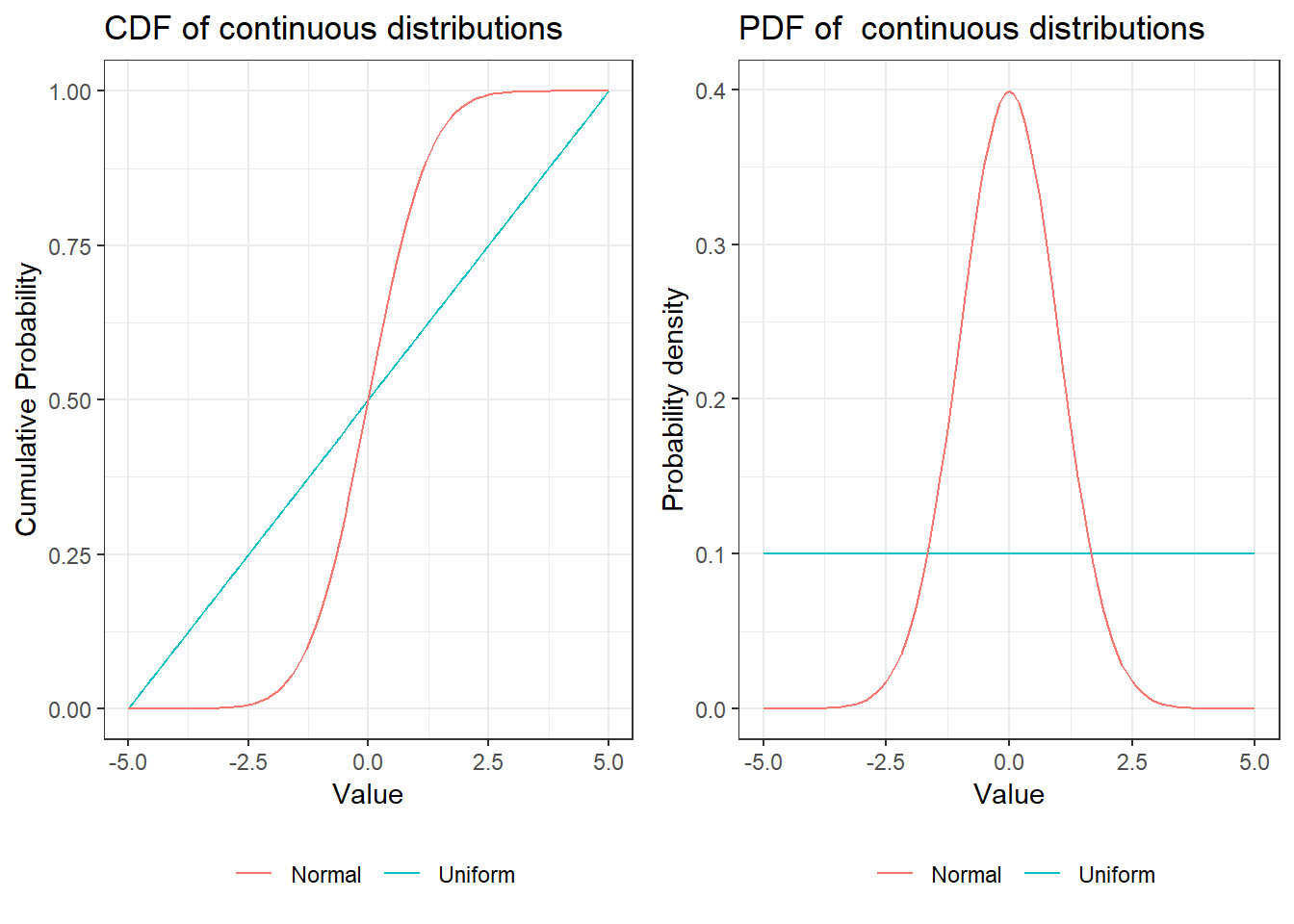
To illustrate the concept of the integral the continuous uniform distribution provides a simple example. As in the discrete case it assigns equal weight to each equally sized interval in the area on which the variable is defined (\([a, b]\)). Why each interval and not each value? Since there are infinitely many values between \(a\) and \(b\) (again due to real numbers) each individual value cannot be assigned a probability small enough for all of the probabilities to sum to \(1\) (which is a basic requirement of a probability). Thus we can only assign a probability to an interval, e.g. \([0, 0.001]\), of which only finitely many exist between \(a\) and \(b\), e.g. \(a = -2\) and \(b = 1\). In this example there exist \(3,000\) intervals of values \([x, x + 0.001]\). Since we are dealing with intervals the probability density can be thought of as the area under the PDF for a given interval or the sum of the areas of very small intervals within the chosen interval.
The PDF is defined as
\[ f_X(x) = \frac{1}{b-a} \text{ if } x \in [a, b], \ 0 \text{ otherwise} \]
That is, the weight \(\frac{1}{b-a}\) is assign to values in the interval of interest and all other values have weight \(0\). As already mentioned all values between \(a\) and \(b\) have to be considered. Thus, in order to calculate the expected value and the variance we have to integrate over \(x\).
\[ \mathbb{E}[X] = ∫_a^b x * \frac{1}{b-a} dx = \frac{b+a}{2} \]
If you plug in \(a = 1\) in the formula above you can see the relation to the discrete uniform distribution and the similar role of integral and summation. Notice also how the expectation operator “translates” to the integral. For the expectation of \(X\) we integrate over all \(x\), the possible realizations of \(X\), weighted by the PDF of \(X\). Now, in order to get the variance we want to calculate the expected squared deviation from the expected value.
\[\begin{align*} Var(X) &= \mathbb{E}\left[(X - \mathbb{E}[X])^{2} \right] = \mathbb{E}\left[\left(X - \frac{b+a}{2}\right)^2\right] \\ &= ∫_a^b \left(x - \frac{b+a}{2}\right)^2 * \frac{1}{b-a} dx = \frac{(b-a)^2}{12} \end{align*}\]
Clearly the Uniform distribution can be used whenever we want to model a population in which all possible outcomes are equally likely.
8.1.2.3.2 Normal distribution
The normal distribution is probably the most widely known one. Its PDF is the famous bell curve. It has two parameters \(\mu\), and \(\sigma^2\). \(\mu\) is the mean and \(\sigma^2\) the variance of the distribution. In the case of \(\mu = 0,\ \sigma^2 = 1\) it is called the standard normal distribution.
The Normal distribution has a few nice properties. It is symmetric around the mean which is nice whenever we want to express the believe that values are less likely the further we get away from the mean but we do not care in which direction. In addition, it can be used to approximate many other distributions including the Binomial distribution under certain conditions (see Central Limit Theorem). The normal distribution can be standardized, i.e. given any random normal variable, \(X\sim N(\mu, \sigma^2)\), we can get a standard normal variable \(Y \sim N(0, 1)\) where \(Y = \frac{X - \mu}{\sigma}\). This means that we can perform calculations using the standard normal distribution and then recover the results for any normal distribution since for a standard normal \(Y\sim N(0,1)\) we can get to any \(X \sim N(\mu, \sigma^{2})\) by defining \(X = \mu + \sigma * Y\) by just rearranging the formula above. In the application below you can see the PDF and CDF of the normal distribution and set a mean and a standard deviation. Try to get an intuition about why this simple transformation works. First change only the mean and observe that the shape of the PDF stays the same and its location is shifted. Starting from a normal distribution with \(μ = 0\) and setting \(\mu = 4\) is equivalent to adding \(4\) to each value (see table of percentiles). Similarly changing the standard deviation from \(σ = 1\) to \(σ = 2,\ 3,\ 4, \dots\) is equivalent to multiplying each value with \(2,\ 3,\ 4, \dots\).
The normal PDF is defined as
\[ f(x | μ, σ) = \frac{1}{\sqrt{2πσ^{2}}} e^{-\frac{1}{2}\frac{(x-\mu)^2}{σ^2}} \]
The first part \(\left(\frac{1}{\sqrt{2\piσ^2}}\right)\) scales the density down at each point as the standard deviation is increased because \(\sigma\) is in the denominator. When you increase the standard deviation in the application above you will see that the density gets lower on the whole range. Intuitively the total mass of \(1\) needs to be distributed over more values and is thus less in each region. The second part \(\left(e^{-\frac{1}{2}\frac{(x-μ)^2}{\sigma^2}}\right)\) re-scales regions based on how far they are away from the mean due to the \((x-\mu)^2\) part. Notice that values further away from the mean are re-scaled more due to this. The negative sign in the exponent means that the scaling is downward. \(\sigma^2\) in the denominator tells us that this scaling is reduced for higher \(\sigma^2\) and “stronger” for lower \(\sigma^2\). In other words: as \(\sigma\) is increased regions further away from the mean get more probability density. If the standard deviation is set to \(1\) for example there is almost no mass for values that deviate from the mean by more than \(2\). However, if we set \(\sigma = 10\) the 75th percentile is at \(6.75\). That is, 25% of values lie above that value. Equivalently, if we take the integral from \(6.75\) to \(∞\) we will get \(0.25\). Remember that the integral is just the surface area under the curve in that interval. This is also equivalent to saying that if we draw from a normal distribution with \(\mu=0,\ \sigma = 10\) the probability of getting at least \(6.75\) is 25%.
The CDF is defined as
\[ P(X \leq x) = \frac{1}{\sqrt{2 \pi σ^2}} \int_{-∞}^x e^{-\frac{1}{2}\frac{-(t-μ)^2}{σ^2}} dt \]
Notice that this is just the integral of the density up to a point \(x\).
When using the Normal distribution in R one has to specify the standard deviation \(\sigma\) rather than the variance \(\sigma^2\). Of course sometimes it is easier to pass sqrt(variance) instead of typing in the standard deviation. For example if \(Var(X) = 2\) then \(SD(X) = \sqrt{2} = 1.41421356\dots\) and it is easier to call rnorm(10, 0, sqrt(2)) to generate 10 random numbers from a Normal distribution with \(\mu = 0, \sigma^2 = 2\).
8.1.2.3.3 \(\chi^2\) Distribution
The \(\chi^2\) (“Chi-Squared”) distribution has only one parameter, its degrees of freedom. The exact meaning of degrees of freedom will be discussed later when we are talking about hypothesis testing. Roughly, they give the number of independent points of information that can be used to estimate a statistic. Naming the parameter of the \(\chi^2\) distribution degrees of freedom reflects its importance for hypothesis testing. That is the case since many models assume the data to be normally distributed and the \(\chi^2\) distribution is closely related to the normal distribution. Explicitly if \(X \sim N(0, 1)\) then \(X^2 \sim \chi^2(1)\). That is, if we have one random variable with standard normal distribution and square it, we get a \(\chi^2\) random variable with \(1\) degree of freedom. How to exactly count the variables that go into a specific statistic will be discussed at a later point. If multiple squared independent standard normal variables are summed up the degrees of freedom increase accordingly.
\[ Q = ∑_{i = 1}^k X_i^2,\ X_{i} \sim N(0,1) \Rightarrow Q \sim \chi^2(k) \]
That is, if we square \(k\) normal variables and sum them up the result is a \(\chi^2\) variable with \(k\) degrees of freedom
Calculating the expected value, using the properties of the standard normal distribution, is simple.
Let \(X \sim N(0,1)\). Then \(Var(X) = \mathbb{E}[X^{2}] - \mathbb{E}[X]^2 = \sigma^2 = 1\). Also, \(\mathbb{E}[X] = \mu = 0\). Therefore, \(\mathbb{E}[X^{2}] = 1\). Thus, the expected value of one squared standard normal variable is \(1\). If we sum \(k\) independent normal variables we get
\[ \mathbb{E}[Q] = \sum_{i = 1}^k \mathbb{E}[X^{2}] = \sum_{i = 1 }^k 1 = k \]
The derivation of the variance is a bit more involved because it involves calculating
\[ \mathbb{E}[Q^{2}] = \mathbb{E}\left[\left(X^{2}\right)^2\right] = \mathbb{E}[X^{4}] \]
where \(Q\sim \chi^2(1)\) and \(X \sim N(0,1)\). However, above we claimed that the Normal distribution has only two parameters, \(\mu,\text{ and } \sigma^2\), for which we only need \(\mathbb{E}[X]\) and \(\mathbb{E}[X^{2}]\) to fully describe the Normal distribution. These are called the first and second moments of the distribution. Equivalently, \(\mathbb{E}[X^{4}]\) is the \(4^{th}\) moment. We can express the \(4^th\) moment in terms of the second moment for any variable that follows a Normal distribution. \(\mathbb{E}[X^{4}] = 3 * \sigma^2\) for any Normal variable and thus \(\mathbb{E}[X^{4}] = 3\) for Standard Normal variables. Therefore, \(\mathbb{E}[Q^{2}] = 3 - \mathbb{E}[Q]^2 = 2\) for \(Q \sim \chi^2(1)\). In general \(Var(Q) = 2k\) for \(Q \sim \chi^2(k)\) due to the variance sum law which states that the variance of a sum of independent variables is equal to the sum of the variances. Notice that this does not hold if the variables are not independent, which is why the independence of the Normal variables that go into the \(\chi^2\) distribution has been emphasized.
8.1.2.4 t-Distribution
Another important distribution for hypothesis testing is the t-distribution, also called Student’s t-distribution. It is the distribution of the location of the mean of a sample from the normal distribution relative to the “true” mean (\(\mu\)). Like the \(\chi^2\) distribution it also has only one parameter called the degrees of freedom. However, in this case the degrees of freedom are the number of draws from the normal distribution minus 1. They are denoted by the Greek letter nu (\(\nu\)). We take \(n\) draws from a Normal distribution with mean \(\mu\) and standard deviation \(\sigma^2\) and let \(\bar X = \frac{1}{n} \sum_{i = 1}^n x_i\) the sample mean and \(S^{2} = \frac{1}{n-1}\sum_{i = 1}^n (x_i - \bar X)^2\) the sample variance. Then
\[ \frac{\bar X - \mu}{S/ \sqrt{n}} \]
has a t-distribution with \(\nu = n-1\) degrees of freedom. Why \(n-1\) and not \(n\) as in the \(\chi^2\) distribution? Recall that when constructing a \(\chi^2(k)\) variable we sum up \(k\) independent standard normally distributed variables but we have no intermediate calculations with these variables. In the case of the t-Distribution we “lose” a degree of freedom due to the intermediary calculations. We can notice this by multiplying and dividing the formula above by \(\sigma\), the “true” variance of the \(x_i\).
\[\begin{align*} & \frac{\bar X - \mu}{S/ \sqrt{n}} \\ =& \frac{\bar X - \mu}{S/ \sqrt{n}} \frac{\frac{1}{\sigma/\sqrt{n}}}{\frac{1}{\sigma/\sqrt{n}}} = \frac{(\bar X - \mu)/(\sigma/\sqrt{n})}{\frac{(S/\sqrt{n})}{(\sigma/\sqrt{n})}}\\ =& \frac{(\bar X - \mu)/(\sigma/\sqrt{n})}{\frac{S}{\sigma}}\\ =& \frac{(\bar X - \mu)/(\sigma/\sqrt{n})}{\sqrt{S^2/\sigma^2}} \end{align*}\]
Now recall the definition of \(S^2 = \frac{1}{n-1} \sum_{i=1}^n (x_i - \bar X)^2\) which is the sum of \(n-1\) independent normally distributed variables, divided by \(n-1\). Only \(n-1\) are independent since given an mean computed from \(n\) variables only \(n-1\) can be chosen arbitrarily.
Let \(\bar X(n) = \frac{1}{n} \sum_{i=1}^n x_i\) Then
\[ x_n = \bar X(n) - \sum_{i = 1}^{n-1} x_i \]
and thus \(x_n\) is not independent.
We already know the distribution of \(n-1\) squared standard normally distributed variables. We introduced the \(\sigma\) term in order to normalize the variable. Therefore the denominator is
\[ \sqrt{\frac{\chi^2_{n-1}}{(n-1)}} \]
Notice that as the degrees of freedom approach infinity the t-Distribution becomes the Standard Normal Distribution.
8.1.2.5 F-Distribution
The F-Distribution is another derived distribution which is important for hypothesis testing. It can be used to compare the variability (i.e. variance) of two populations given that they are normally distributed and independent. Given samples from these two populations the F-Distribution is the distribution of
\[ \frac{S^2_1 / S^2_2}{\sigma^2_1/\sigma^2_2} = \frac{S^2_1/\sigma^{2}_1}{S^2_2/\sigma^2_2} \]
As shown above both the numerator and the denominator are \(\chi^2(n-1)\) divided by the degrees of freedom
\[ F_{n-1, m-1} = \frac{\chi^2_{n-1}/(n-1)}{\chi^2_{m-1}/(m-1)} \]
8.1.3 Appendix
8.1.3.1 Derivation of the varaince of the binomial distribution
Notice that the sum follows this pattern for \(n = 1\) and any appropriate \(p\):
\[ Var(X_i) = p * (1-p)^2 + (1-p) * p^2 \]
If we expand the squared term and simplify:
\[\begin{align*} Var(X_i) &= p * (1 - 2*p + p^2) + p^2 - p^3 \\ &= p - 2*p^2 + p^3 + p^2 - p^3 \\ &= p - p^2 \end{align*}\]
What happens if we change the number of coins to \(2\) and keep \(p=0.8\)?
\[ Var(X_2) = 0.8 * 0.2^2 + 0.2 * 0.8^2 + 0.8 * 0.2^2 + 0.2 * 0.8^2 = 2 * (0.8 * 0.2^2 + 0.2 * 0.8^2) = 2 * (0.8 - 0.8^2) = 0.32 \]
Since increasing \(n\) further simply adds more of the same terms we can easily adapt the general formula above for any appropriate \(n\) and \(p\):
\[ Var(X_i) = n * (p-p^2) \]
Equivalently this formula can be written as:
\[ n * (p - p^2) = np - np^2 = np * (1-p) = Var(X_i) \]
8.2 Regression
8.2.1 Linear regression
This chapter contains the Appendix for the chapter on regression analysis.
In order to understand the coefficients in the multiple regression we can derive them separately. We have already seen that in the univariate case:
\[ \hat{\beta_1}=\frac{COV_{XY}}{s_x^2} \]
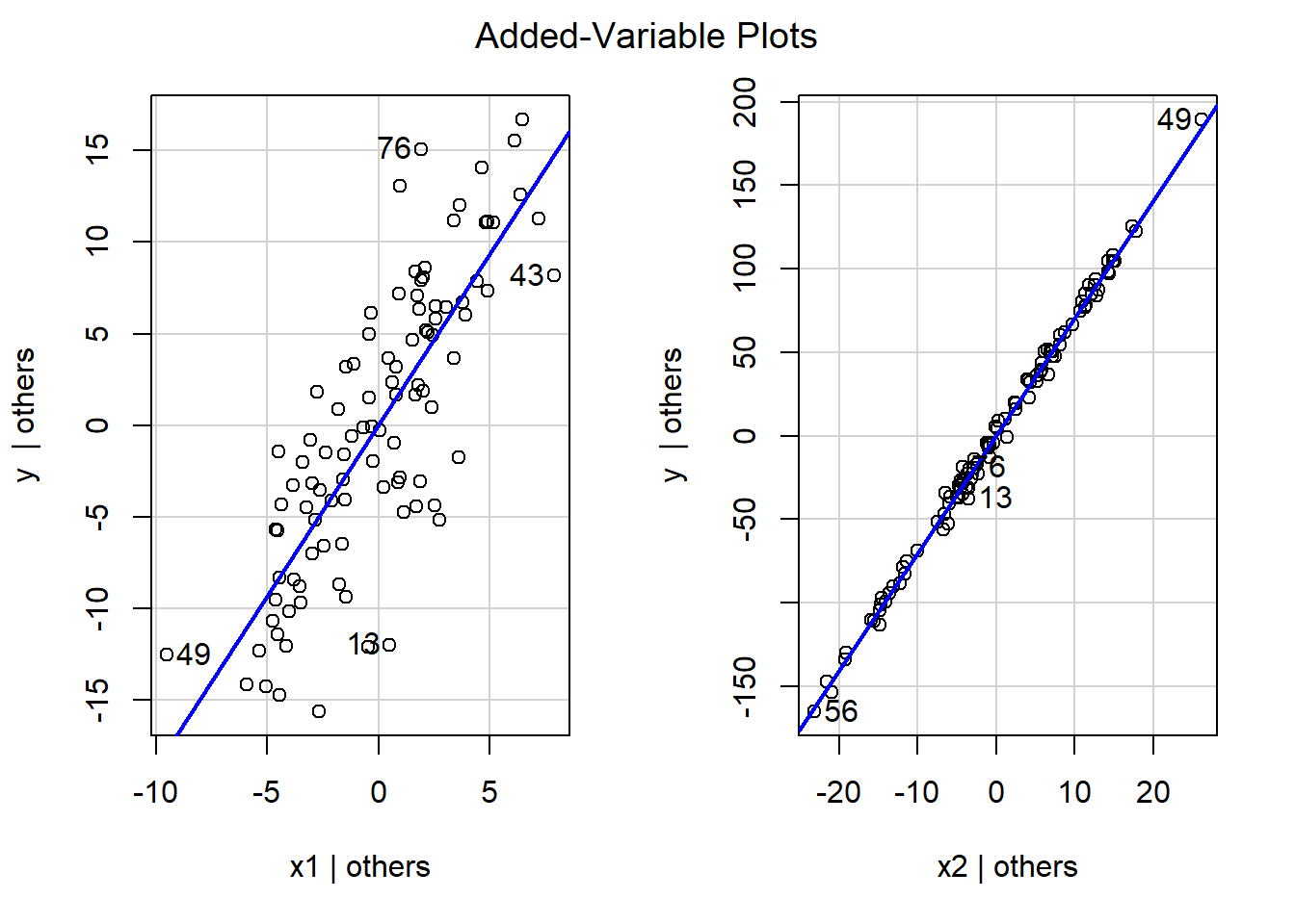
We have also seen that we can isolate the partial effect of a single variable in a multiple regression. Specifically, we can calculate the coefficient of the i-th variable as
\[ \hat{\beta_{i}} = {COV(\tilde{Y_{i}}, \tilde{X_{i}}) \over V(\tilde{X_i})} \]
where \(\tilde{Y_{i}}\) is the residual from the regression of \(Y\) on all variables except for the i-th and \(\tilde{X_i}\) is the residual from the regression of \(X_i\) on all other variables. Let’s illustrate this with an example.
We have added some randomness through the rnorm command so the coefficients are not exactly as we set them but close. Clearly x1 and x2 have partial influence on y.
##
## Call:
## lm(formula = y ~ x1 + x2)
##
## Residuals:
##      Min       1Q   Median       3Q      Max
## -12.9482  -2.4227   0.3595   3.1597  11.5191
##
## Coefficients:
##             Estimate Std. Error t value            Pr(>|t|)
## (Intercept) 49.88523    1.08974   45.78 <0.0000000000000002 ***
## x1           1.86227    0.13939   13.36 <0.0000000000000002 ***
## x2           7.03624    0.04617  152.41 <0.0000000000000002 ***
## ---
## Signif. codes:  0 '***' 0.001 '**' 0.01 '*' 0.05 '.' 0.1 ' ' 1
##
## Residual standard error: 4.706 on 97 degrees of freedom
## Multiple R-squared:  0.9998, Adjusted R-squared:  0.9998
## F-statistic: 3.036e+05 on 2 and 97 DF,  p-value: < 0.00000000000000022
To see the partial effect of x1 we run regressions for x1 on x2, as well as y on x2 and obtain the residuals \(\tilde{x1}\) and \(\tilde{x2}\). Notice that x1 is highly correlated with x2.
##
## Call:
## lm(formula = x1 ~ x2)
##
## Residuals:
##     Min      1Q  Median      3Q     Max
## -9.5397 -2.7946  0.3462  2.1645  7.9205
##
## Coefficients:
##              Estimate Std. Error t value            Pr(>|t|)
## (Intercept) -6.620773   0.419971  -15.77 <0.0000000000000002 ***
## x2           0.323652   0.007106   45.55 <0.0000000000000002 ***
## ---
## Signif. codes:  0 '***' 0.001 '**' 0.01 '*' 0.05 '.' 0.1 ' ' 1
##
## Residual standard error: 3.41 on 98 degrees of freedom
## Multiple R-squared:  0.9549, Adjusted R-squared:  0.9544
## F-statistic: 2074 on 1 and 98 DF, p-value: < 0.00000000000000022We can use the residuals to create the partial plots as seen above.
# This is the same as avPlot
ggplot(data.frame(y = tildeY1, x = tildeX1), aes(x = x, y = y)) +
  geom_point(shape = 1) +
  geom_smooth(method = 'lm', se = FALSE, color = "red") +
  labs(y = "y | others", x = "x1 | others") +
  theme_bw()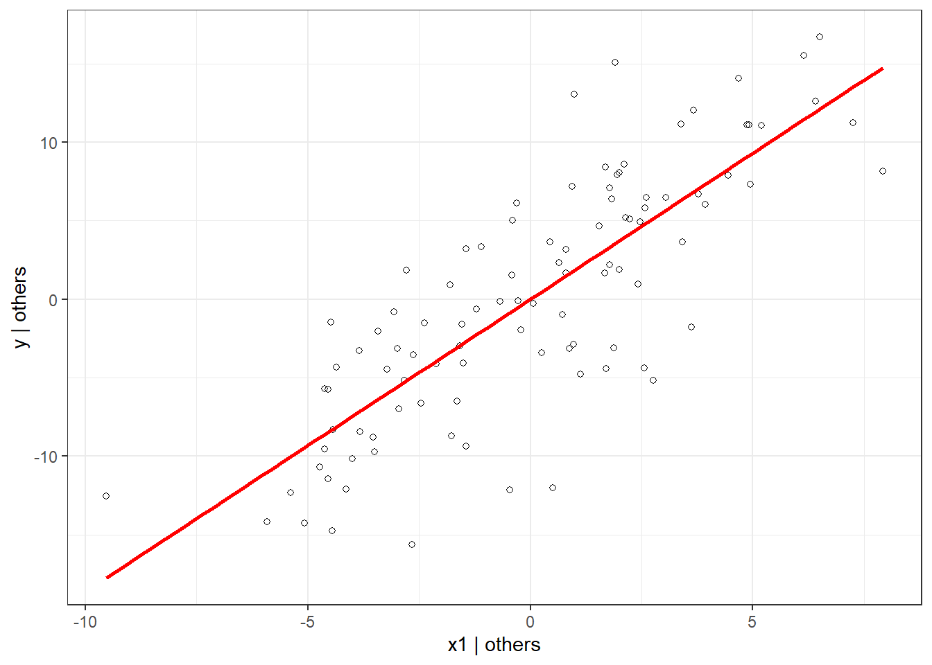
And the regression of the residuals of y on x1 yields the same coefficient as in the original regression (minus the rounding errors).
# This is the same coefficient as in the original regression
summary(lm(tildeY1~tildeX1 - 1)) # -1 since we want no intercept
##
## Call:
## lm(formula = tildeY1 ~ tildeX1 - 1)
##
## Residuals:
## Min 1Q Median 3Q Max
## -12.9482 -2.4227 0.3595 3.1597 11.5191
##
## Coefficients:
## Estimate Std. Error t value Pr(>|t|)
## tildeX1 1.862 0.138 13.5 <0.0000000000000002 ***
## ---
## Signif. codes: 0 '***' 0.001 '**' 0.01 '*' 0.05 '.' 0.1 ' ' 1
##
## Residual standard error: 4.658 on 99 degrees of freedom
## Multiple R-squared: 0.6479, Adjusted R-squared: 0.6443
## F-statistic: 182.2 on 1 and 99 DF, p-value: < 0.00000000000000022## [1] "Coefficient using the partial covariance:"## [1] 1.8622748.2.2 Logistic regression
8.2.2.1 Maximum likelihood estimation
For non-linear models we cannot turn to linear algebra to solve for the unknown parameters. However, we can use a statistical method called maximum likelihood estimation (MLE). Given observed data and an assumption about their distribution we can estimate for which parameter values the observed data is most likely to occur. We do this by calculating the joint log likelihood of the observations given a choice of parameters (more on that below). Next, we change our parameter values a little bit and see if the joint log likelihood improved. We keep doing that until we cannot find better parameter values anymore (that is we have reached the maximum likelihood). In the following example we have a histogram of a data set which we assume to be normally distributed. You can now try to find the best parameter values by changing the mean and the variance. Recall that the normal distribution is fully described by just those two parameters. In each step the log likelihood is automatically calculated. The maximum likelihood so far is shown as the high score and the line in the lower graph shows the development of the log likelihood for the past couple of tries.
8.2.2.2 Estimation of the parameters \(\beta_i\)
Let’s return to the model to figure out how the parameters \(\beta_i\) are estimated. In the data we observe the \(y_i\), the outcome variable that is either \(0\) or \(1\), and the \(x_{i,j}\), the predictors for each observation. In addition, by using the logit model we have assumed the following functional form.
\[ P(y_i = 1) = \frac{1}{1 + e^{-(\beta_0 + \beta_1 * x_{1,i} + \beta_2 * x_{2,i} + ... +\beta_m * x_{m,i})}} \]
So far we have looked at estimating the \(\beta_i\) with R but have not discussed how that works. In contrast to linear models (e.g. OLS) we cannot rely on linear algebra to solve for \(\beta_i\) since the function is now non-linear. Therefore, we turn to a methodology called maximum likelihood estimation. Basically, we try out different \(\beta_i\) and choose the combination that best fits the observed data. In other words: choose the combination of \(\beta_i\) that maximize the likelihood of observing the given data set. For each individual we have information about the binary outcome and the predictors. For those whose outcome is \(1\) we want to choose the \(\beta_i\) such that our predicted probability of the outcome (\(P(y_i = 1)\)) is as close to \(1\) as possible. At the same time, for those whose outcome is \(0\) we would like the prediction (\(P(y_i = 1)\)) to be as close to \(0\) as possible. Therefore, we “split” the sample into two groups (outcome \(1\) and outcome \(0\)). For the first group each individual has the probability function shown above which we want to maximize for this group. For the other group we would need to minimize the joint probability since we want our prediction to be as close to \(0\) as possible. Alternatively we can easily transform the probability to \(P(y_i = 0)\) which we can then maximize. Since probabilities add up to \(1\) and we only have two possible outcomes \(P(y_i = 0) = 1 - P(y_i = 1)\). This is convenient because now we can calculate the joint likelihood of all observations and maximize a single function. We assume that the observations are independent from each other and thus the joint likelihood is just the product of the individual probabilities. Thus for the group of \(n_1\) individuals with outcome \(1\) we have the joint likelihood
\[ \prod_{i=1}^{n_1} {1 \over 1 + e^{-(\beta_0 + \beta_1 * x_{1,i} + \beta_2 * x_{2,i} + ... +\beta_m * x_{m,i})}} \]
For the second group of \(n_2\) individuals with outcome \(0\) we get the joint likelihood
\[ \prod_{j=1}^{n_{2}} 1 - {1 \over 1 + e^{-(\beta_0 + \beta_1 * x_{1,i} + \beta_2 * x_{2,i} + ... +\beta_m * x_{m,i})}} \]
In order to find the optimal \(\beta_i\) we need to combine to two groups into one joint likelihood function for all observations. We can once again do that by multiplying them with each other. However, now we need to add an indicator in order to determine in which group the observation is.
\[ \prod_{k = 1}^{n_1 + n_2} \left({1 \over 1 + e^{-(\beta_0 + \beta_1 * x_{1,i} + \beta_2 * x_{2,i} + ... +\beta_m * x_{m,i})}}\right)^{y_i} \times \left( 1 - {1 \over 1 + e^{-(\beta_0 + \beta_1 * x_{1,i} + \beta_2 * x_{2,i} + ... +\beta_m * x_{m,i})}}\right)^{1-y_i} \]
The indicators \((\cdot)^{y_i}\) and \((\cdot)^{1-y_i}\) select the appropriate likelihood. To illustrate this consider an individual with outcome \(y_j = 1\)
\[ \begin{align*} &\left({1 \over 1 + e^{-(\beta_0 + \beta_1 * x_{1,j} + \beta_2 * x_{2,j} + ... +\beta_m * x_{m,j})}}\right)^{y_j} \times \left( 1 - {1 \over 1 + e^{-(\beta_0 + \beta_1 * x_{1,j} + \beta_2 * x_{2,j} + ... +\beta_m * x_{m,j})}}\right)^{1-y_j}\\ =&\left({1 \over 1 + e^{-(\beta_0 + \beta_1 * x_{1,j} + \beta_2 * x_{2,j} + ... +\beta_m * x_{m,j})}}\right)^{1} \times \left( 1 - {1 \over 1 + e^{-(\beta_0 + \beta_1 * x_{1,j} + \beta_2 * x_{2,j} + ... +\beta_m * x_{m,j})}}\right)^{0}\\ =&{1 \over 1 + e^{-(\beta_0 + \beta_1 * x_{1,j} + \beta_2 * x_{2,j} + ... +\beta_m * x_{m,j})}} \times 1\\ =&{1 \over 1 + e^{-(\beta_0 + \beta_1 * x_{1,j} + \beta_2 * x_{2,j} + ... +\beta_m * x_{m,j})}} \end{align*} \]
Equivalently for an individual with outcome \(y_s = 0\):
\[ \begin{align*} &\left({1 \over 1 + e^{-(\beta_0 + \beta_1 * x_{1,i} + \beta_2 * x_{2,i} + ... +\beta_m * x_{m,i})}}\right)^{y_i} \times \left( 1 - {1 \over 1 + e^{-(\beta_0 + \beta_1 * x_{1,i} + \beta_2 * x_{2,i} + ... +\beta_m * x_{m,i})}}\right)^{1-y_i}\\ =&\left({1 \over 1 + e^{-(\beta_0 + \beta_1 * x_{1,j} + \beta_2 * x_{2,j} + ... +\beta_m * x_{m,j})}}\right)^{0} \times \left( 1 - {1 \over 1 + e^{-(\beta_0 + \beta_1 * x_{1,j} + \beta_2 * x_{2,j} + ... +\beta_m * x_{m,j})}}\right)^{1}\\ =&1\times \left( 1 - {1 \over 1 + e^{-(\beta_0 + \beta_1 * x_{1,j} + \beta_2 * x_{2,j} + ... +\beta_m * x_{m,j})}}\right)^{1}\\ =& 1 - {1 \over 1 + e^{-(\beta_0 + \beta_1 * x_{1,j} + \beta_2 * x_{2,j} + ... +\beta_m * x_{m,j})}} \end{align*} \]
8.2.2.3 Example
Consider an experiment in which we want to find out whether a person will listen to the full song or skip it. Further, assume that the genre of the song is the only determining factor of whether somebody is likely to skip it or not. Each individual has rated the genre on a scale from 1 (worst) to 10 (best). Our model looks as follows:
\[ P(\text{skipped}_i) = {1 \over 1 + e^{-(\beta_0 + \beta_1 \text{rating}_i)}} \]
The probability that individual \(i\) will skip a song is the logistic function with \(X = \beta_0 + \beta_1 * \text{rating}_i\), where \(\text{rating}_i\) is individual \(i\)’s rating of the genre of the song. Since we assume independence of individuals we can write the joint likelihood as
\[ \prod_{i=1}^{N} \left({1 \over 1 + e^{-(\beta_0 + \beta_1 \text{rating}_i)}}\right)^{y_i} \times \left(1- {1 \over 1 + e^{-(\beta_0 + \beta_1 \text{rating}_i)}}\right)^{(1-y_i)} \]
Notice that \(y_i\) is either equal to one or to zero. So for each individual only one of the two parts is not equal to one (recall that any real number to the power of 0 is equal to 1). The the part left of the plus sign is “looking at” individuals who skipped the song given their rating and the right part is looking at individuals who did not skip the song given their rating. For the former we want the predicted probability of skipping to be as high as possible. For the latter we want the predicted probability of not skipping to be as high as possible and thus write \(1 - {1 \over 1+ e^{-(\beta_0 + \beta_1 \text{rating}_i)}}\). This is convenient since we can now maximize a single function. Another way to simplify the calculation and make it computationally feasible is taking the logarithm. This will ensure that extremely small probabilities can still be processed by the computer (see this illustration).
Manually applying this in R would looks as follows. We begin by simulating some data. ratingGenre is a vector of 10000 randomly generated numbers between 1 and 10. pSkip will be a vector of probabilities generated by applying the logistic function to our linear model, with the parameters \(\beta_0 = 1\) and \(\beta_1 = -0.3\).
ratingGenre <- sample(1:10, size = 10000, replace = TRUE)
linModel <- 1 - 0.3 * ratingGenre
pSkip <- 1/(1+exp(-linModel))
Now we have to sample whether a user skipped a song or not, based on their probability of skipping. The resulting vector skipped is composed of 0s and 1s and indicates whether or not a person skipped a song.
skipped <- 1:length(pSkip)
for(i in 1:length(pSkip)){
  skipped[i] <- sample(c(1, 0), size = 1, prob = c(pSkip[i], 1-pSkip[i]))
}
Our simulated data now looks as follows:
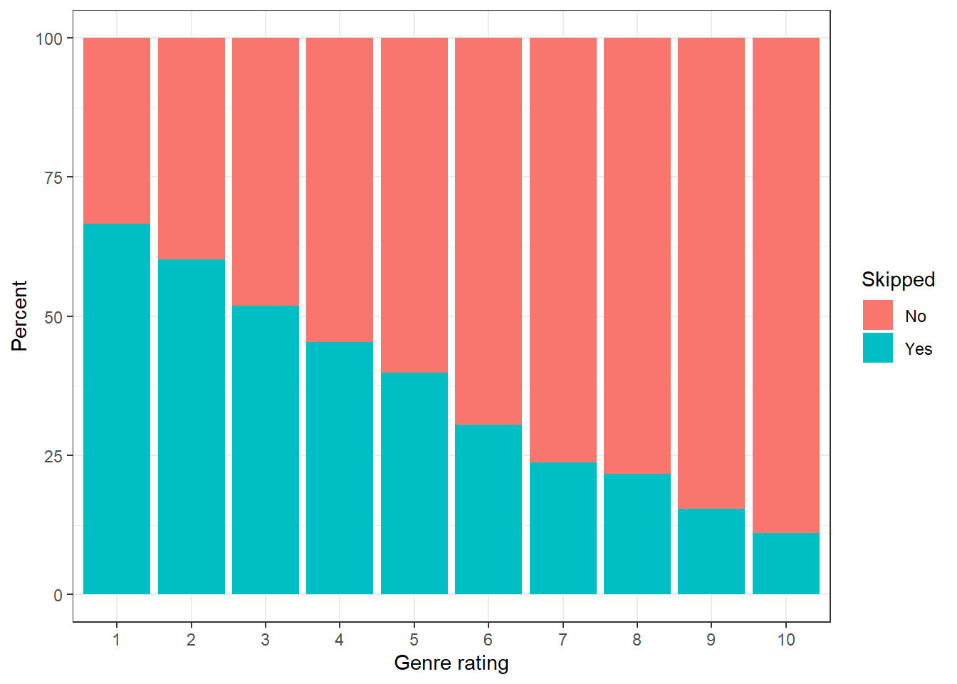
Figure 8.1: Percent of songs skipped as a function of the genre rating
The visualization shows that an increase in genreRating leads to a decrease in the probability of a song being skipped. Now we want to perform maximum likelihood estimation and see how close we get to the true parameter values. To achieve this, we need a function that, given a value for \(\beta_0\) and \(\beta_1\), gives us the value of the log likelihood. The following code defines such a function.
mlEstimate <- function(beta_0, beta_1){
  pred <- 1/(1+exp(-(beta_0 + beta_1 * ratingGenre)))
  loglik <- skipped * log(pred) + (1-skipped) * log(1 - pred)
  sum(loglik)
}
The log likelihood function has the following form.
Figure 8.2: Plot of the log likelihood function
As you can see, the maximum of the log likelihood function lies around -0.3, 1, the true parameter values. Now we need to find an algorithm that finds the combination of \(\beta_0\) and \(\beta_1\) that optimizes this function. There are multiple ways to go about this. The glm() function uses the built-in optimization function optim(). While we could do the same, we will use a slightly different approach to make the process more intuitive. We are going to employ something called grid maximization. Basically, we make a list of all plausible combinations of parameter values and calculate the log likelihood for each combination. Then we simply select the parameter combination that has the highest log likelihood.
prob_beta_0 and prob_beta_1 are now vectors that contain 100 plausible values for each parameter.
prob_beta_0 <- seq(0.5, 1.5, length.out = 100)
prob_beta_1 <- seq(-1, 0, length.out = 100)

# Print one vector as an example
prob_beta_0
## [1] 0.5000000 0.5101010 0.5202020 0.5303030 0.5404040 0.5505051 0.5606061
## [8] 0.5707071 0.5808081 0.5909091 0.6010101 0.6111111 0.6212121 0.6313131
## [15] 0.6414141 0.6515152 0.6616162 0.6717172 0.6818182 0.6919192 0.7020202
## [22] 0.7121212 0.7222222 0.7323232 0.7424242 0.7525253 0.7626263 0.7727273
## [29] 0.7828283 0.7929293 0.8030303 0.8131313 0.8232323 0.8333333 0.8434343
## [36] 0.8535354 0.8636364 0.8737374 0.8838384 0.8939394 0.9040404 0.9141414
## [43] 0.9242424 0.9343434 0.9444444 0.9545455 0.9646465 0.9747475 0.9848485
## [50] 0.9949495 1.0050505 1.0151515 1.0252525 1.0353535 1.0454545 1.0555556
## [57] 1.0656566 1.0757576 1.0858586 1.0959596 1.1060606 1.1161616 1.1262626
## [64] 1.1363636 1.1464646 1.1565657 1.1666667 1.1767677 1.1868687 1.1969697
## [71] 1.2070707 1.2171717 1.2272727 1.2373737 1.2474747 1.2575758 1.2676768
## [78] 1.2777778 1.2878788 1.2979798 1.3080808 1.3181818 1.3282828 1.3383838
## [85] 1.3484848 1.3585859 1.3686869 1.3787879 1.3888889 1.3989899 1.4090909
## [92] 1.4191919 1.4292929 1.4393939 1.4494949 1.4595960 1.4696970 1.4797980
## [99] 1.4898990 1.5000000Next we create a data frame that contains all possible combinations of prob_beta_0 and prob_beta_1. The expand.grid() function does exactly that.
With the apply() function we can calculate the log likelihood for each value in the data frame. Note that the params data frame now has a now column containing the log likelihood.
Next we simply find the highest log likelihood value and the associated parameter values.
As you can see, our method comes pretty close to the true parameter values. For comparison, here is the same model calculated with the glm() function.
##
## Call:
## glm(formula = skipped ~ ratingGenre, family = binomial(link = "logit"))
##
## Deviance Residuals:
##     Min       1Q   Median       3Q      Max
## -1.4895  -0.8638  -0.5806   1.0095   2.0606
##
## Coefficients:
##              Estimate Std. Error z value            Pr(>|z|)
## (Intercept)  1.009642   0.046579   21.68 <0.0000000000000002 ***
## ratingGenre -0.300527   0.008365  -35.93 <0.0000000000000002 ***
## ---
## Signif. codes:  0 '***' 0.001 '**' 0.01 '*' 0.05 '.' 0.1 ' ' 1
##
## (Dispersion parameter for binomial family taken to be 1)
##
##     Null deviance: 13140  on 9999  degrees of freedom
## Residual deviance: 11632  on 9998  degrees of freedom
## AIC: 11636
##
## Number of Fisher Scoring iterations: 3
8.2.2.3.1 Sum of LN vs Product
To illustrate why the natural log (ln) is important for computations with numbers close to zero (such as joint probabilities), we create a vector of fictitious probabilities and multiply them with each other. As we can see, already a small number of values close to 0 will lead to their product being erroneously interpreted as being 0. If we are only interested in comparing magnitude (as in the case of likelihoods) we can safely apply the ln, since it is a monotonically increasing function and will thus not change the ranking.
probs <- c(0.000001, 0.000001, 0.000001, 0.000001, 0.000001, 0.000001, 0.000001,
           0.000001, 0.000001, 0.000001, 0.000001, 0.000001, 0.000001, 0.000001,
           0.000001, 0.000001, 0.000001, 0.000001, 0.000001, 0.000001, 0.000001,
           0.000001, 0.000001, 0.000001, 0.000001, 0.000001, 0.000001, 0.000001,
           0.000001, 0.000001, 0.000001, 0.000001, 0.000001, 0.000001, 0.000001,
           0.000001, 0.000001, 0.000001, 0.000001, 0.000001, 0.000001, 0.000001,
           0.000001, 0.000001, 0.000001, 0.000001, 0.000001, 0.000001, 0.000001,
           0.000001, 0.000001, 0.000001, 0.000001, 0.000001, 0.000001, 0.000001)
prod(probs)
## [1] 0## [1] -773.6686probs2 <- rbind(probs, probs, probs, probs, probs,
probs, probs, probs, probs, probs) # now 10 times as many values
lProbs2 <- log(probs2)
sum(lProbs2)## [1] -7736.686