3 Data import and export
Before you can start your analytics in R, you first need to import the data you wish to perform the analytics on. You will often be faced with different types of data formats (usually produced by some other statistical software like SPSS or Excel or a text editor). Fortunately, R is fairly flexible with respect to the sources from which data may be imported and you can import the most common data formats into R with the help of a few packages. R can, among others, handle data from the following sources (based on “R in Action” by R. Kabacoff):
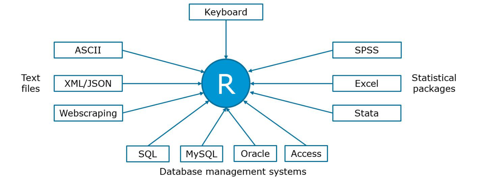
Figure 3.1: Data import
In the previous chapter, we saw how we may use the keyboard to input data in R. In the following sections, we will learn how to import data from text files and other statistical software packages.
3.1 Getting data for this course
Most of the datasets we will be working with in this course will be stored in text files (i.e., .dat, .txt, .csv). There are two ways for you to obtain access to the datasets:
3.1.1 Directly import datasets from GitHub (recommended)
All datasets we will be working with are stored in a repository on GitHub (similar to other cloud storage services such as Dropbox). If you know the location, where the files are stored, you may conveniently load the data directly from GitHub into R using the read.table() function. The header=TRUE argument indicates that the first line of data represents the header, i.e., it contains the names of the columns. The sep="\t"-argument specifies the delimiter (the character used to separate the columns), which is a TAB in this case.
test_data <- read.table("https://raw.githubusercontent.com/IMSMWU/Teaching/master/MRDA2017/test_data.dat",
    sep = "\t", header = TRUE)
3.1.2 Download and import datasets from “Learn@WU”
It is also possible to download the data from the respective folder on the “Learn@WU” platform, placing it in the working directory and importing it from there. However, this requires an additional step to download the file manually first. If you chose this option, please remember to put the data file in the working directory first. If the import is not working, check your working directory setting using getwd(). Once you placed the file in the working directory, you can import it using the same command as above. Note that the file must be given as a character string (i.e., in quotation marks) and has to end with the file extension (e.g., .csv, .tsv, etc.).
test_data <- read.table(test_file, header = TRUE)3.2 Import data created by other software packages
Sometimes, you may need to import data files created by other software packages, such as Excel or SPSS. In this section we will use the readxl and haven packages to do this. To import a certain file you should first make sure that the file is stored in your current working directory. You can list all file names in your working directory using the list.files() function. If the file is not there, either copy it to your current working directory, or set your working directory to the folder where the file is located using setwd("/path/to/file"). This tells R the folder you are working in. Remember that you have to use / instead of \ to specify the path (if you use Windows paths copied from the explorer they will not work). When your file is in your working directory you can simply enter the filename into the respective import command. The import commands offer various options. For more details enter ?read_excel, ?read_spss after loading the packages.
list.files()  #lists all files in the current working directory
# setwd('/path/to/file') #may be used to change the
# working directory to the folder that contains the
# desired file

# import excel files
library(readxl)  #load package to import Excel files
excel_sheets("test_data.xlsx")
test_data_excel <- read_excel("test_data.xlsx", sheet = "mrda_2016_survey")  # 'sheet=x'' specifies which sheet to import
head(test_data_excel)

library(haven)  #load package to import SPSS files
# import SPSS files
test_data_spss <- read_sav("test_data.sav")
head(test_data_spss)
The import of other file formats works in a very similar way (e.g., Stata, SAS). Please refer to the respective help-files (e.g., ?read_dta, ?read_sas …) if you wish to import data created by other software packages.
3.3 Export data
Exporting to different formats is also easy, as you can just replace “read” with “write” in many of the previously discussed functions (e.g. write.table(file_name)). This will save the data file to the working directory. To check what the current working directory is you can use getwd(). By default, the write.table(file_name)function includes the row number as the first variable. By specifying row.names = FALSE, you may exclude this variable since it doesn’t contain any useful information.
write.table(test_data, "testData.dat", row.names = FALSE,
    sep = "\t")  #writes to a tab-delimited text file
write.table(test_data, "testData.csv", row.names = FALSE,
    sep = ",")  #writes to a comma-separated value file
write_sav(test_data, "my_file.sav")
3.4 Import data from the Web
3.4.1 Scraping data from websites
Sometimes you may come accross interesting data on websites that you would like to analyse. Reading data from websites is possible in R, e.g., using the rvest package. Let’s assume you would like to read a table that lists the population of different countries from this Wikipedia page. It helps to first inspect the structure of the website (e.g., using tools like SelectorGadget), so you know which elements you would like to extract. In this case it is fairly obvious that the data are stored in a table for which the associated html-tag is <table>. So let’s read the entire website using read_html(url) and filter all tables using read_html(html_nodes(...,"table")).
library(rvest)
url <- "https://en.wikipedia.org/wiki/List_of_countries_and_dependencies_by_population"
population <- read_html(url)
population <- html_nodes(population, "table")
print(population)
## {xml_nodeset (3)}
## [1] <table class="plainlinks metadata ambox ambox-move" role="presentati ...
## [2] <table class="wikitable sortable" style="text-align:right">\n<tr>\n< ...
## [3] <table class="nowraplinks hlist collapsible autocollapse navbox-inne ...The output shows that there are two tables on the website and the first one appears to contain the relevant information. So let’s read the first table using the html_table() function. Note that population is of class “list”. A list is a vector that has other R objects (e.g., other vectors, dataframes, matrices, etc.) as its elements. If we want to access the data of one of the elements, we have to use two square brackets on each side instead of just one (e.g., population[[1]] gets us the first table from the list of tables on the website; the argument fill = TRUE ensures that empty cells are replaced with missing values when reading the table).
population <- population[[2]] %>% html_table(fill = TRUE)
head(population)  #checks if we scraped the desired data
You can see that population is read as a character variable because of the commas.
class(population$Population)## [1] "character"If we wanted to use this variable for some kind of analysis, we would first need to convert it to numeric format using the as.numeric() function. However, before we can do this, we can use the gsub() function, which replaces all matches of a string. In our case, we would like to replace the commas (",") with nothing ("").
population$Population <- as.numeric(gsub(",", "", population$Population))  #convert to numeric
head(population)  #checks if we scraped the desired data
Now the variable is of type “numeric” and could be used for analysis.
class(population$Population)## [1] "numeric"3.4.2 Scraping data from APIs
3.4.2.1 Scraping data from APIs directly
Reading data from websites can be tricky since you need to analyze the page structure first. Many web-services (e.g., Facebook, Twitter, YouTube) actually have application programming interfaces (API’s), which you can use to obtain data in a pre-structured format. JSON (JavaScript Object Notation) is a popular lightweight data-interchange format in which data can be obtained. The process of obtaining data is visualized in the following graphic (see also http://broadcast.oreilly.com/2009/07/use-apis-to-do-research.html):
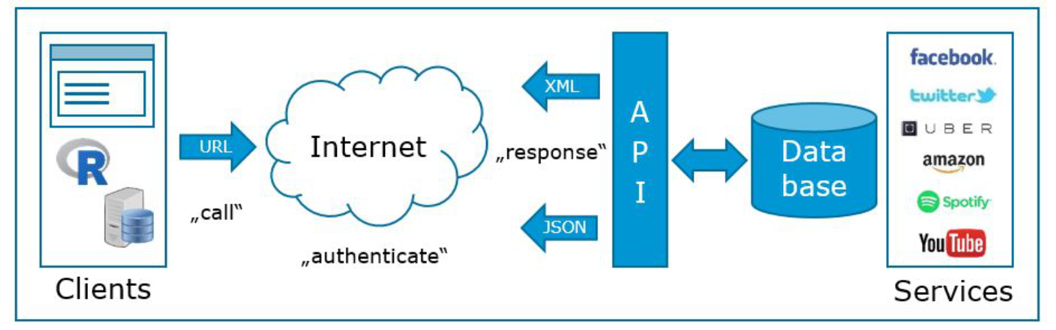
Figure 3.2: Obtaining data from APIs
The process of obtainig data from APIs consists of the following steps:
- Identify an API that has enough data to be relevant and reliable (e.g., www.programmableweb.com has >12,000 open web APIs in 63 categories).
- Request information by calling (or, more technically speaking, creating a request to) the API (e.g., R, python, php or JavaScript).
- Receive response messages, which is usually in JavaScript Object Notation (JSON) or Extensible Markup Language (XML) format.
- Write a parser to pull out the elements you want and put them into a of simpler format
- Store, process or analyze data according the marketing research question.
Let’s assume that you would like to obtain population data again. The World Bank has an API that allows you to easily obtain this kind of data. The details are usually provided in the API reference, e.g., here. You simply “call” the API for the desired information and get a structured JSON file with the desired key-value pairs in return. For example, the population for Austria from 1960 to 2016 can be obtained using this call. The file can be easily read into R using the fromJSON()-function from the jsonlite-package. Again, the result is a list and the second element ctrydata[[2]] contains the desired data, from which we select the “value” and “data” columns using the square brackets as usual [,c("value","date")]
library(jsonlite)
url <- "http://api.worldbank.org/countries/AT/indicators/SP.POP.TOTL/?date=1960:2016&format=json&per_page=100"  #specifies url
ctrydata <- fromJSON(url)  #parses the data
str(ctrydata)
## List of 2
## $ :List of 4
## ..$ page : int 1
## ..$ pages : int 1
## ..$ per_page: chr "100"
## ..$ total : int 57
## $ :'data.frame': 57 obs. of 5 variables:
## ..$ indicator:'data.frame': 57 obs. of 2 variables:
## .. ..$ id : chr [1:57] "SP.POP.TOTL" "SP.POP.TOTL" "SP.POP.TOTL" "SP.POP.TOTL" ...
## .. ..$ value: chr [1:57] "Population, total" "Population, total" "Population, total" "Population, total" ...
## ..$ country :'data.frame': 57 obs. of 2 variables:
## .. ..$ id : chr [1:57] "AT" "AT" "AT" "AT" ...
## .. ..$ value: chr [1:57] "Austria" "Austria" "Austria" "Austria" ...
## ..$ value : chr [1:57] "8747358" "8633169" "8541575" "8479375" ...
## ..$ decimal : chr [1:57] "0" "0" "0" "0" ...
## ..$ date : chr [1:57] "2016" "2015" "2014" "2013" ...head(ctrydata[[2]][, c("value", "date")]) #checks if we scraped the desired data3.4.2.2 Scraping data from APIs via R packages
An even more convenient way to obtain data from web APIs is to use existing R packages that someone else has already created. There are R packages available for various web-services. For example, the gtrendsR package can be used to conveniently obtain data from the Google Trends page. The gtrends() function is easy to use ans returns a list of elements (e.g., “interest over time”, “interest by city”, “related topics”), which can be inspected using the ls() function. The following example can be used to obtain data for the search term “data science” in the US between September 1 and October 6:
library(gtrendsR)
google_trends <- gtrends("data science", geo = c("US"),
    gprop = c("web"), time = "2017-09-01 2017-10-06")
ls(google_trends)
## [1] "interest_by_city" "interest_by_country" "interest_by_dma"
## [4] "interest_by_region" "interest_over_time" "related_queries"
## [7] "related_topics"head(google_trends$interest_over_time)