4 Introduction to Statistical Inference
This chapter will provide you with a basic intuition on statistical inference. As marketing researchers we are usually faced with “imperfect” data in the sense that we cannot collect all the data we would like. Imagine you are interested in the average amount of time WU students spend listening to music every month. Ideally, we could force all WU students to fill out our survey. Realistically we will only be able to observe a small fraction of students (maybe 500 out of the \(25.000+\)). With the data from this small fraction at hand, we want to make an inference about the true average listening time of all WU students. We are going to start with the assumption that we know everything. That is, we first assume that we know all WU students’ listening times and analyze the distribution of the listening time in the entire population. Subsequently, we are going to look at the uncertainty that is introduced by only knowing some of the students’ listening times (i.e., a sample from the population) and how that influences our analysis.
You can download the corresponding R-Code here
4.1 If we knew it all
Assume there are \(25,000\) students at WU and every single one has kindly provided us with the hours they listened to music in the past month. In this case, we know the true mean (\(49.93\) hours) and the true standard deviation (SD = \(10.02\)) and thus we can easily summarize the entire distribution. Since the data follows a normal distribution, roughly 95% of the values lie within 2 standard deviations from the mean, as the following plot shows:
library(tidyverse)
library(ggplot2)
library(latex2exp)
set.seed(321)
hours <- rnorm(25000, 50, 10)

ggplot(data.frame(hours)) +
  geom_histogram(aes(hours), bins = 50, fill = 'white', color = 'black') +
  labs(title = "Histogram of listening times",
       subtitle = TeX(sprintf("Population mean ($\\mu$) = %.2f; population standard deviation ($\\sigma$) = %.2f",round(mean(hours),2),round(sd(hours),2))),
       y = 'Number of students',
       x = 'Hours') +
  theme_bw() +
  geom_vline(xintercept = mean(hours), size = 1) +
  geom_vline(xintercept = mean(hours)+2*sd(hours), colour = "red", size = 1) +
  geom_vline(xintercept = mean(hours)-2*sd(hours), colour = "red", size = 1) +
  geom_segment(aes(x = mean(hours), y = 1100, yend = 1100, xend = (mean(hours) - 2*sd(hours))), lineend = "butt", linejoin = "round",
     size = 0.5, arrow = arrow(length = unit(0.2, "inches"))) +
  geom_segment(aes(x = mean(hours), y = 1100, yend = 1100, xend = (mean(hours) + 2*sd(hours))), lineend = "butt", linejoin = "round",
     size = 0.5, arrow = arrow(length = unit(0.2, "inches"))) +
  annotate("text", x = mean(hours) + 28, y = 1100, label = "Mean + 2 * SD" )+
  annotate("text", x = mean(hours) -28, y = 1100, label = "Mean - 2 * SD" )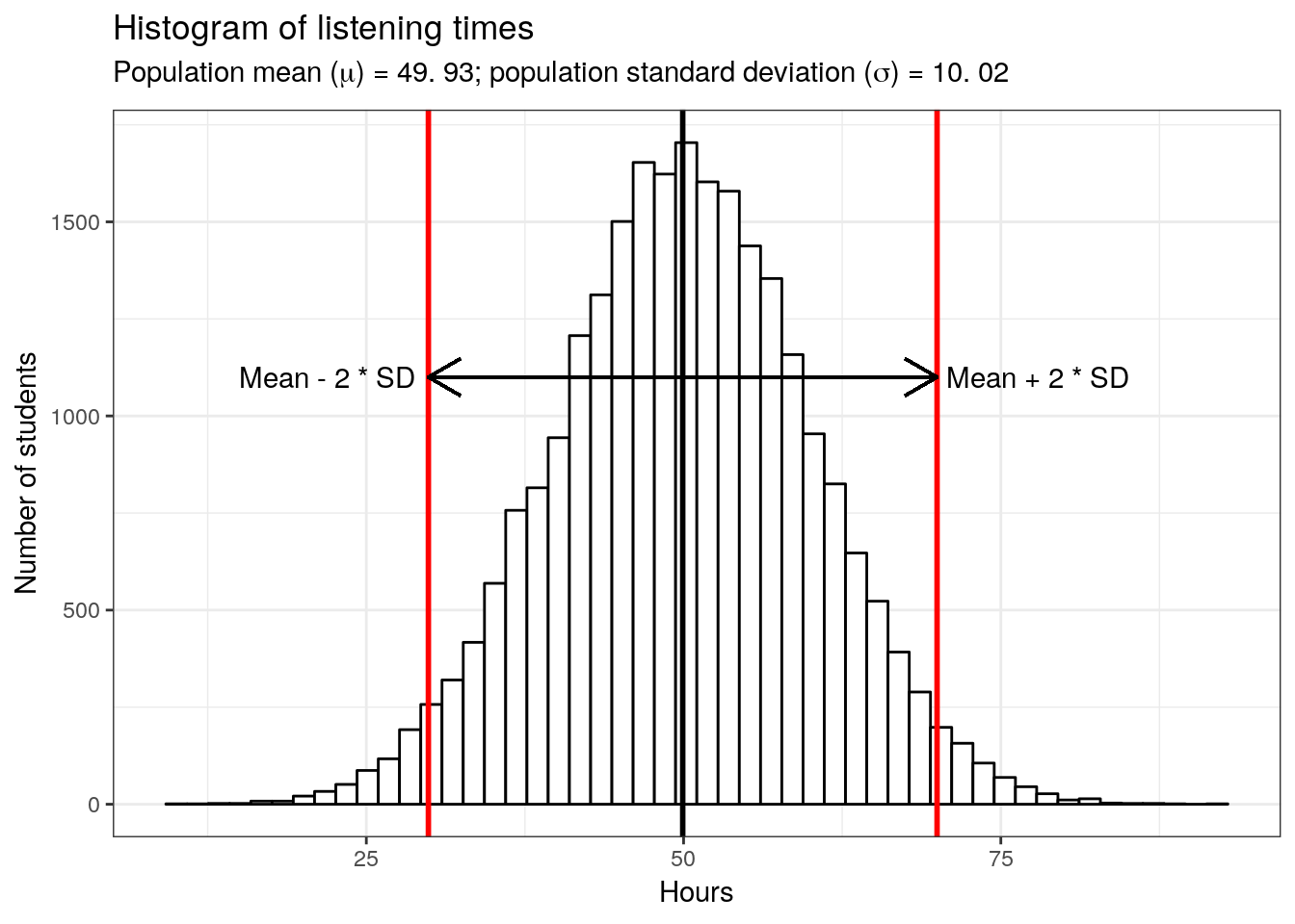
In this case, we refere to all WU students as the population. In general, the population is the entire group we are interested in. This group does not have to necessarily consist of people, but could also be companies, stores, animals, etc.. The parameters of the distribution of population values (in hour case: “hours”) are called population parameters. As already mentioned, we do not usually know population parameters but use inferential statistics to infer them based on our sample from the population, i.e., we measure statistics from a sample (e.g., the sample mean \(\bar x\)) to estimate population parameters (the population mean \(\mu\)). Here, we will use the following notation to refer to either the population parameters or the sample statistic:
| Variable | Sample statistic | Population parameter |
|---|---|---|
| Size | n | N |
| Mean | \(\bar{x} = {1 \over n}\sum_{i=1}^n x_i\) | \(\mu = {1 \over N}\sum_{i=1}^N x_i\) |
| Variance | \(s^2 = {1 \over n-1}\sum_{i=1}^n (x_i-\bar{x})^2\) | \(\sigma^2 = {1 \over N}\sum_{i=1}^N (x_i-\mu)^2\) |
| Standard deviation | \(s = \sqrt{s^2}\) | \(\sigma = \sqrt{\sigma^2}\) |
| Standard error | \(SE_{\bar x} = {s \over \sqrt{n}}\) | \(\sigma_{\bar x} = {\sigma \over \sqrt{n}}\) |
4.1.1 Sampling from a known population
In the first step towards a realistic research setting, let us take one sample from this population and calculate the mean listening time. We can simply sample the row numbers of students and then subset the hours vector with the sampled rownumbers. The sample() function will be used to draw a sample of size 100 from the population of 25,000 students, and one student can only be drawn once (i.e., replace = FALSE). The following plot shows the distribution of listening times for our sample.
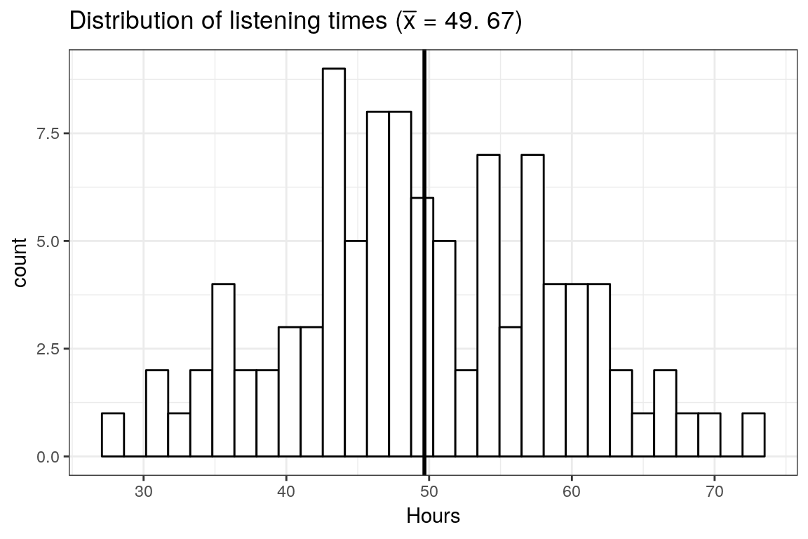
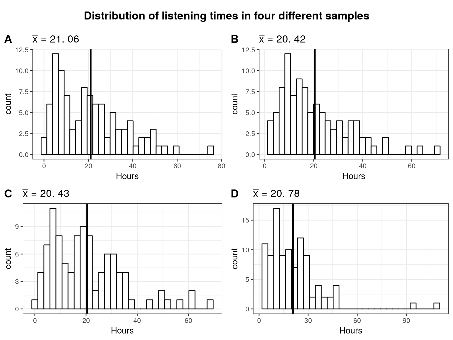
Observe that in this first draw the mean (\(\bar x =\) 49.67) is quite close to the actual mean ($= $ 49.93). It seems like the sample mean is a decent estimate of the population mean. However, we could just be lucky this time and the next sample could turn out to have a different mean. Let us continue by looking at four additional random samples, consisting of 100 students each. The following plot shows the distribution of listening times for the four different samples from the population.
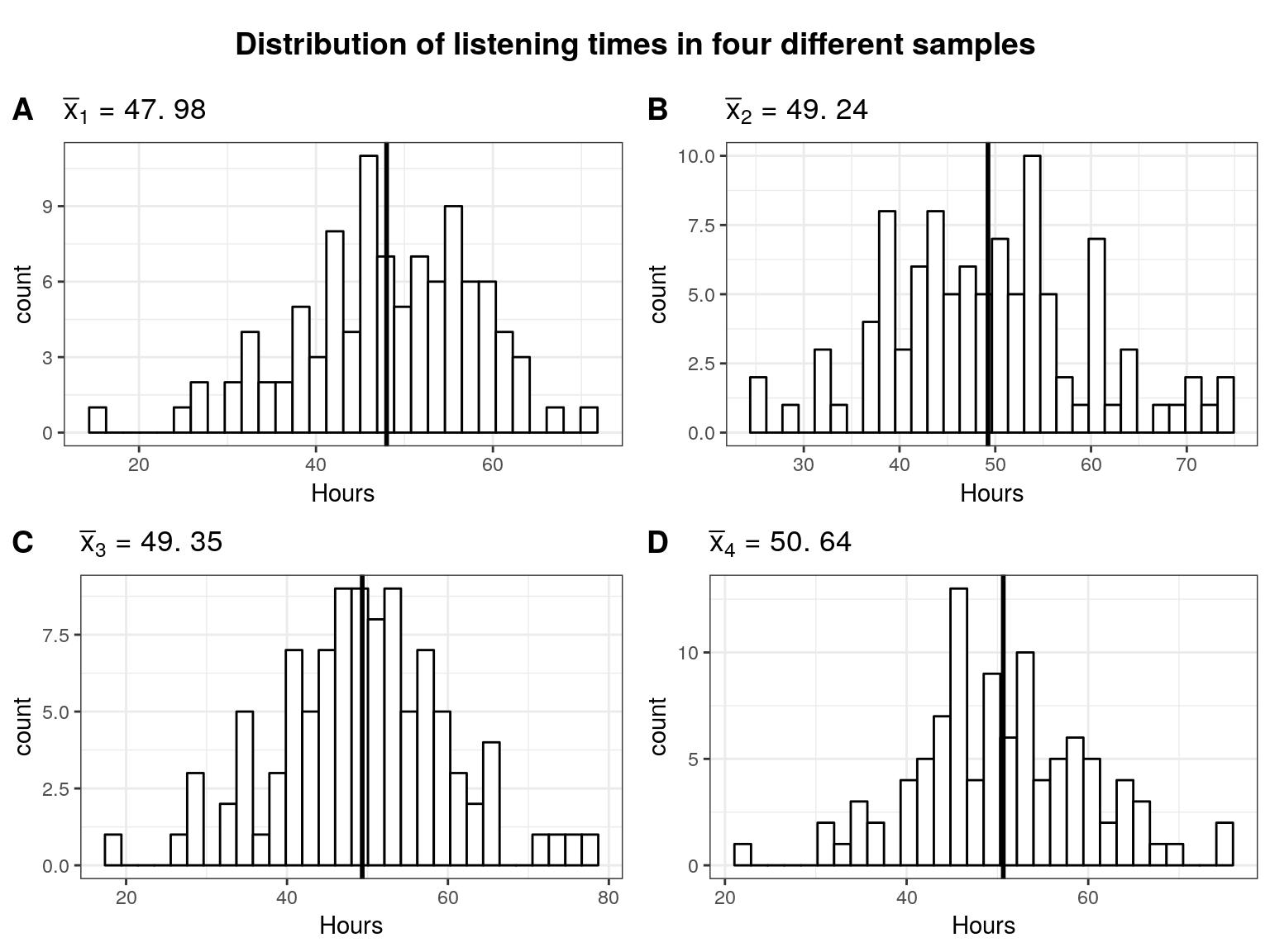
It becomes clear that the mean is slightly different for each sample. This is referred to as sampling variation and it is completely fine to get a slightly different mean every time we take a sample. We just need to find a way of expressing the uncertainty associated with the fact that we only have data from one sample, because in a realistic setting you are most likely only going to have access to a single sample.
So in order to make sure that the first draw is not just pure luck and the sample mean is in fact a good estimate for the population mean, let us take many (e.g., \(20,000\)) different samples from the population. That is, we repeatedly draw 100 students randomly from the population without replacement (that is, once a student has been drawn she or he is removed from the pool and cannot be drawn again) and calculate the mean of each sample. This will show us a range within which the sample mean of any sample we take is likely going to be. We are going to store the means of all the samples in a matrix and then plot a histogram of the means to observe the likely values.
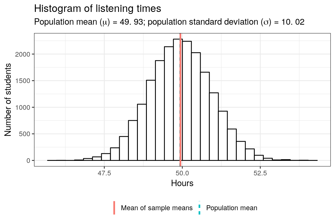
As you can see, on average the sample mean (“mean of sample means”) is extremely close to the population mean, despite only sampling \(100\) people at a time. This distribution of sample means is also referred to as sampling distribution of the sample mean. However, there is some uncertainty, and the means are slightly different for the different samples and range from 45.95 to 54.31.
4.1.2 Standard error of the mean
Due to the variation in the sample means shown in our simulation, it is never possible to say exactly what the population mean is based on a single sample. However, even with a single sample we can infer a range of values within which the population mean is likely contained. In order to do so, notice that the sample means are approximately normally distributed. Another interesting fact is that the mean of sample means (i.e., 49.94) is roughly equal to the population mean (i.e., 49.93). This tells us already that generally the sample mean is a good approximation of the population mean. However, in order to make statements about the expected range of possible values, we would need to know the standard deviation of the sampling distribution. The formal representation of the standard deviation of the sample means is
\[ \sigma_{\bar x} = {\sigma \over \sqrt{n}} \]
where \(\sigma\) is the population SD and \(n\) is the sample size. \(\sigma_{\bar{x}}\) is referred to as the Standard Error of the mean and it expresses the variation in sample means we should expect given the number of observations in our sample and the population SD. That is, it provides a measure of how precisely we can estimate the population mean from the sample mean.
4.1.2.1 Sample size
The first thing to notice here is that an increase in the number of observations per sample \(n\) decreases the range of possible sample means (i.e., the standard error). This makes intuitive sense. Think of the two extremes: sample size \(1\) and sample size \(25,000\). With a single person in the sample we do not gain a lot of information and our estimate is very uncertain, which is expressed through a larger standard deviation. Looking at the histogram at the beginning of this chapter showing the number of students for each of the listening times, clearly we would get values below \(25\) or above \(75\) for some samples. This is way farther away from the population mean than the minimum and the maximum of our \(100\) person samples. On the other hand, if we sample every student we get the population mean every time and thus we do not have any uncertainty (assuming the population does not change). Even if we only sample, say \(24,000\) people every time, we gain a lot of information about the population and the sample means would not be very different from each other since only up to \(1,000\) people are potentially different in any given sample. Thus, with larger (smaller) samples, there is less (more) uncertainty that the sample is a good approximation of the entire population. The following plot shows the relationship between the sample size and the standard error. Samples of increasing size are randomly drawn from the population of WU students. You can see that the standard error is decreasing with the number of observations.
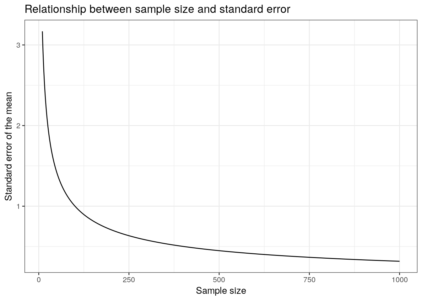
Figure 4.1: Relationship between the sample size and the standard error
The following plots show the relationship between the sample size and the standard error in a slightly different way. The plots show the range of sample means resulting from the repeated sampling process for different sample sizes. Notice that the more students are contained in the individual samples, the less uncertainty there is when estimating the population mean from a sample (i.e., the possible values are more closely centered around the mean). So when the sample size is small, the sample mean can expected to be very different the next time we take a sample. When the sample size is large, we can expect the sample means to be more similar every time we take a sample.
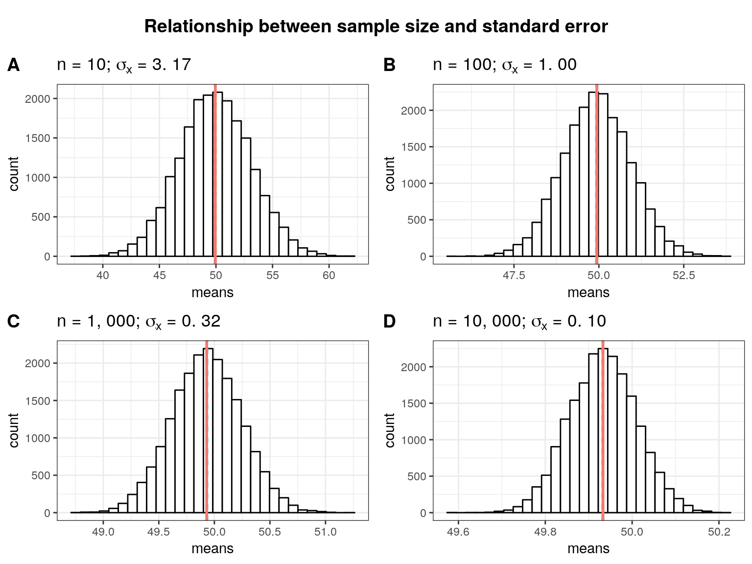
As you can see, the standard deviation of the sample means (\(\sigma_{\bar x}\)) decreases as the sample size increases as a consequence of the reduced uncertainty about the true sample mean when we take larger samples.
4.1.2.2 Population standard deviation
A second factor determining the standard deviation of the distribution of sample means (\(\sigma_{\bar x}\)) is the standard deviation associated with the population parameter (\(\sigma\)). Again, looking at the extremes illustrates this well. If all WU students listened to music for approximately the same amount of time, the samples would not differ much from each other. In other words, if the standard deviation in the population is lower, we expect the standard deviation of the sample means to be lower as well. This is illustrated by the following plots.
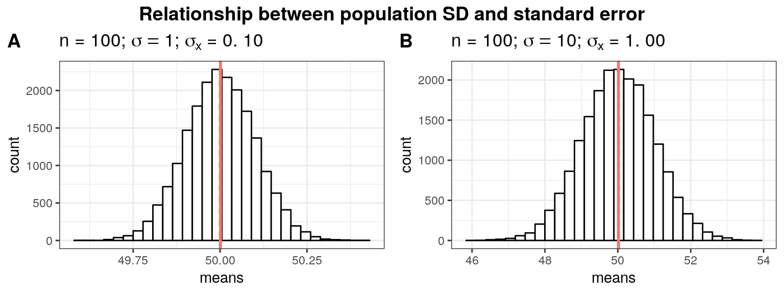
In the first plot (panel A), we assume a much smaller population standard deviation (e.g., \(\sigma\) = 1 instead of \(\sigma\) = 10). Notice how the smaller (larger) the population standard deviation, the less (more) uncertainty there is when estimating the population mean from a sample (i.e., the possible values are more closely centered around the mean). So when the population SD is large, the sample mean can expected to be very different the next time we take a sample. When the population SD is small, we can expect the sample means to be more similar.
4.2 The Central Limit Theorem
The attentive reader might have noticed that the population above was generated using a normal distribution function. It would be very restrictive if we could only analyze populations whose values are normally distributed. Furthermore, we are unable in reality to check whether the population values are normally distributed since we do not know the entire population. However, it turns out that the results generalize to many other distributions. This is described by the Central Limit Theorem.
The central limit theorem states that if (1) the population distribution has a mean (there are examples of distributions that don’t have a mean , but we will ignore these here), and (2) we take a large enough sample, then the sampling distribution of the sample mean is approximately normally distributed. What exactly “large enough” means depends on the setting, but the interactive element at the end of this chapter illustrates how the sample size influences how accurately we can estimate the population parameters from the sample statistics.
To illustrate this, let’s repeat the analysis above with a population from a gamma distribution. In the previous example, we assumed a normal distribution so it was more likely for a given student to spend around 50 hours per week listening to music. The following example depicts the case in which most students spend a similar amount of time listening to music, but there are a few students who very rarely listen to music, and some music enthusiasts with a very high level of listening time. Here is a histogram of the listening times in the population:
set.seed(321)
hours <- rgamma(25000, shape = 2, scale = 10)
ggplot(data.frame(hours)) +
  geom_histogram(aes(x = hours), bins = 30, fill='white', color='black') +
    geom_vline(xintercept = mean(hours), size = 1)  +  theme_bw() +
  labs(title = "Histogram of listening times",
       subtitle = TeX(sprintf("Population mean ($\\mu$) = %.2f; population standard deviation ($\\sigma$) = %.2f",round(mean(hours),2),round(sd(hours),2))),
       y = 'Number of students',
x = 'Hours') 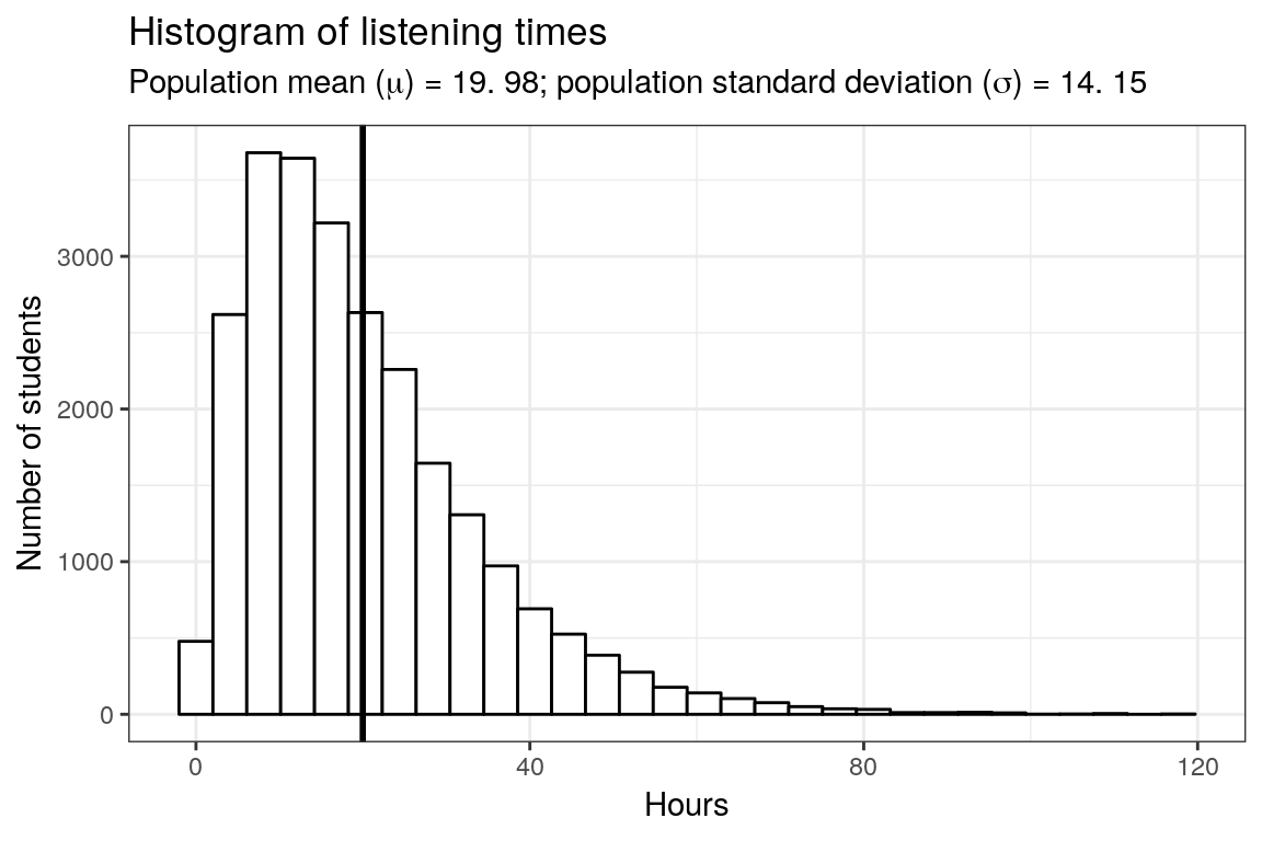
The vertical black line represents the population mean (\(\mu\)), which is 19.98 hours. The following plot depicts the histogram of listening times of four random samples from the population, each consisting of 100 students:
As in the previous example, the mean is slightly different every time we take a sample due to sampling variation. Also note that the distribution of listening times no longer follows a normal distribution as a result of the fact that we now assume a gamma distribution for the population with a positive skew (i.e., lower values more likely, higher values less likely).
Let’s see what happens to the distribution of sample means if we take an increasing number of samples, each drawn from the same gamma population:
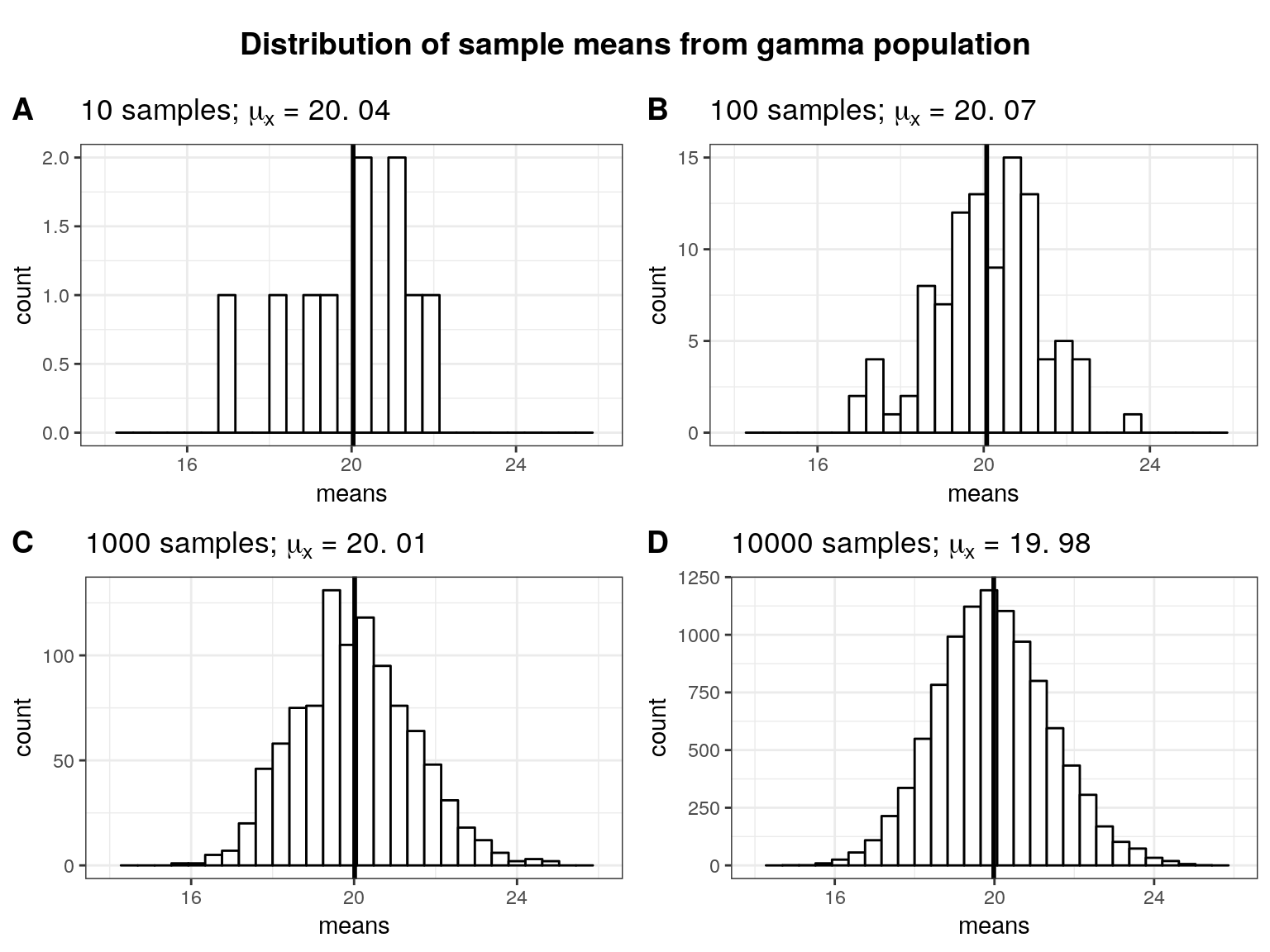
Two things are worth noting: (1) The more (hypothetical) samples we take, the more the sampling distribution approaches a normal distribution. (2) The mean of the sampling distribution of the sample mean (\(\mu_{\bar x}\)) is very similar to the population mean (\(\mu\)). From this we can see that the mean of a sample is a good estimate of the population mean.
In summary, it is important to distinguish two types of variation: (1) For each individual sample that we may take in real life, the standard deviation (\(s\)) is used to describe the natural variation in the data and the data may follow a non-normal distribution. (2) If we would (hypothetically!) repeat the study many times, the sampling distribution of the sample mean follows a normal distribution for large samples sizes (even if data from each individual study are non-normal), and the standard error (\(\sigma_{\bar x}\)) is used to describe the variation between study results. This is an important feature, since many statistical tests assume that the sampling distribution is normally distributed. As we have seen, this does not mean that the data from one particular sample needs to follow a normal distribution.
4.3 Using what we actually know
So far we have assumed to know the population standard deviation (\(\sigma\)). This an unrealistic assumption since we do not know the entire population. The best guess for the population standard deviation we have is the sample standard deviation, denoted \(s\). Thus, the standard error of the mean is usually estimated from the sample standard deviation:
\[ \sigma_{\bar x} \approx SE_{\bar x}={s \over \sqrt{n}} \]
Note that \(s\) itself is a sample estimate of the population parameter \(\sigma\). This additional estimation introduces further uncertainty. You can see in the interactive element below that the sample SD, on average, provides a good estimate of the population SD. That is, the distribution of sample SDs that we get by drawing many samples is centered around the population value. Again, the larger the sample, the closer any given sample SD is going to be to the population parameter and we introduce less uncertainty. One conclusion is that your sample needs to be large enough to provide a reliable estimate of the population parameters. What exactly “large enough” means depends on the setting, but the interactive element illustrates how the remaining values change as a function of the sample size.
We will not go into detail about the importance of random samples but basically the correctness of your estimate depends crucially on having a sample at hand that actually represents the population. Unfortunately, we will usually not notice if the sample is non-random. Our statistics are still a good approximation of “a” population parameter, namely the one for the population that we actually sampled but not the one we are interested in. To illustrate this uncheck the “Random Sample” box below. The new sample will be only from the top \(50\%\) music listeners (but this generalizes to different types of non-random samples).
4.3.1 Confidence Intervals for the Sample Mean
When we try to estimate parameters of populations (e.g., the population mean \(\mu\)) from a sample, the average value from a sample (e.g., the sample mean \(\bar x\)) only provides an estimate of what the real population parameter is. The next time you collect a sample of the same size, you could get a different average. This is sampling variation and it is completely fine to get a slightly different sample mean every time we take a sample as we have seen above. However, this inherent uncertainty about the true population parameter means that coming up with an exact estimate (i.e., a point estimate) for a particular population parameter is really difficult. That is why it is often informative to construct a range around that statistic (i.e., an interval estimate) that likely contains the population parameter with a certain level of confidence. That is, we construct an interval such that for a large share (say 95%) of the sample means we could potentially get, the population mean is within that interval.
Let us consider one random sample of 100 students from our population above.
set.seed(321)
hours <- rgamma(25000, shape = 2, scale = 10)

set.seed(6789)
sample_size <- 100
student_sample <- sample(1:25000, size = sample_size, replace = FALSE)
hours_s <- hours[student_sample]

plot2 <- ggplot(data.frame(hours_s)) +
  geom_histogram(aes(x = hours_s), bins = 30, fill='white', color='black') +
  theme_bw() + xlab("Hours") +
  geom_vline(aes(xintercept = mean(hours_s)), size=1) +
 ggtitle(TeX(sprintf("Random sample; $n$ = %d; $\\bar{x}$ = %.2f; $s$ = %.2f",sample_size,round(mean(hours_s),2),round(sd(hours_s),2))))
plot2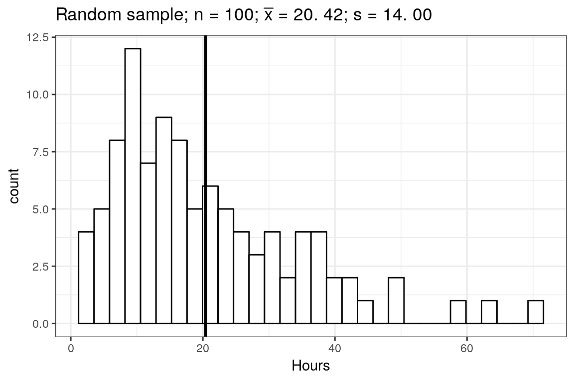
From the central limit theorem we know that the sampling distribution of the sample mean is approximately normal and we know that for the normal distribution, 95% of the values lie within about 2 standard deviations from the mean. Actually, it is not exactly 2 standard deviations from the mean. To get the exact number, we can use the quantile function for the normal distribution qnorm():
qnorm(0.975)## [1] 1.959964We use 0.975 (and not 0.95) to account for the probability at each end of the distribution (i.e., 2.5% at the lower end and 2.5% at the upper end). We can see that 95% of the values are roughly within 1.96 standard deviations from the mean. Since we know the sample mean (\(\bar x\)) and we can estimate the standard deviation of the sampling distribution (\(\sigma_{\bar x} \approx {s \over \sqrt{n}}\)), we can now easily calculate the lower and upper boundaries of our confidence interval as:
\[ CI_{lower} = {\bar x} - z_{1-{\alpha \over 2}} * \sigma_{\bar x} \\ CI_{upper} = {\bar x} + z_{1-{\alpha \over 2}} * \sigma_{\bar x} \]
Here, \(\alpha\) refers to the significance level. You can find a detailed discussion of this point at the end of the next chapter. For now, we will adopt the widely accepted significance level of 5% and set \(\alpha\) to 0.05. Thus, \(\pm z_{1-{\alpha \over 2}}\) gives us the z-scores (i.e., number of standard deviations from the mean) within which range 95% of the probability density lies.
Plugging in the values from our sample, we get:
sample_mean <- mean(hours_s)
se <- sd(hours_s)/sqrt(sample_size)
ci_lower <- sample_mean - qnorm(0.975)*se
ci_upper <- sample_mean + qnorm(0.975)*se
ci_lower
## [1] 17.67089ci_upper## [1] 23.1592such that if we collected 100 samples and computed the mean and confidence interval for each of them, in \(95\%\) of the cases, the true population mean is going to be within this interval between 17.67 and 23.16. This is illustrated in the plot below that shows the mean of the first 100 samples and their confidence intervals:
set.seed(12)
samples <- 100
hours <- rgamma(25000, shape = 2, scale = 10)
means <- matrix(NA, nrow = samples)
for (i in 1:samples){
  student_sample <- sample(1:25000, size = 100, replace = FALSE)
  means[i,] <- mean(hours[student_sample])
}

means_sd <- data.frame(means, lower =  means - qnorm(0.975) * (sd(hours)/sqrt(100)), upper = means + qnorm(0.975) * (sd(hours)/sqrt(100)), y = 1:100)
means_sd$diff <- factor(ifelse(means_sd$lower > mean(hours) | means_sd$upper < mean(hours), 'No', 'Yes'))

ggplot2::ggplot(means_sd, aes(y = y)) +
  scale_y_continuous(breaks = seq(1, 100, by = 1), expand = c(0.005,0.005)) +
  geom_point(aes(x = means, color = diff)) +
  geom_errorbarh(aes(xmin = lower, xmax = upper, color = diff)) +
  geom_vline(xintercept = mean(hours)) +
  scale_color_manual(values = c("red", "black")) +
  guides(color=guide_legend(title="True mean in CI")) +
  theme_bw()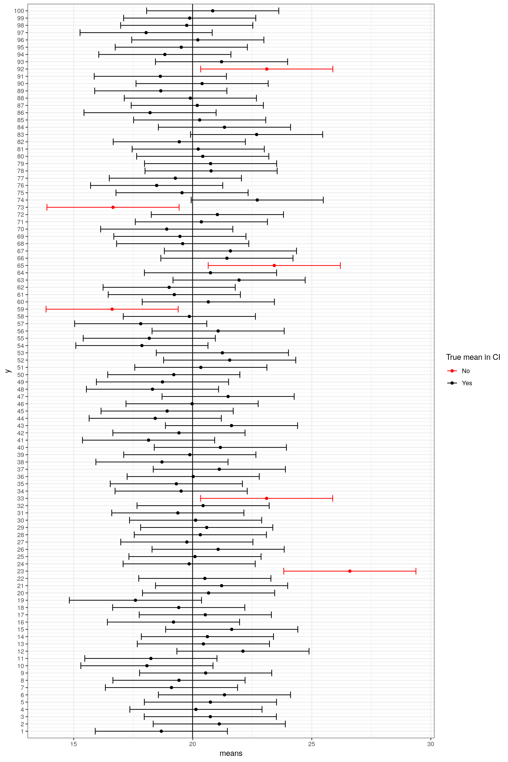
Note that this does not mean that for a specific sample there is a \(95\%\) chance that the population mean lies within its confidence interval. The statement depends on the large number of samples we do not actually draw in a real setting. You can view the set of all possible confidence intervals similarly to the sides of a coin or a die. If we throw a coin many times, we are going to observe head roughly half of the times. This does not, however, exclude the possibility of observing tails for the first 10 throws. Similarly, any specific confidence interval might or might not include the population mean but if we take many samples on average \(95\%\) of the confidence intervals are going to include the population mean.
4.4 Summary
When conducting research, we are (almost) always faced with the problem of not having access to the entire group we are interested in. Therefore, we use sample properties that we have derived in this chapter to do statistical inference based on a single sample. We use statistics of the sample as well as the sample size to calculate the confidence interval of our choice (e.g. \(95\%\)). In practice most of this is done for us, so you won’t need to do this by hand. With a sample at hand, we need to choose the appropriate test and a null hypothesis. How this is done will be discussed in the next chapter.